This simulation of the shearing of a lap joint illustrates the use of general contact in Abaqus/Standard.
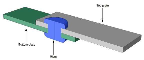
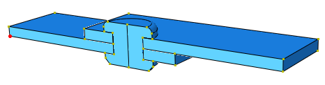
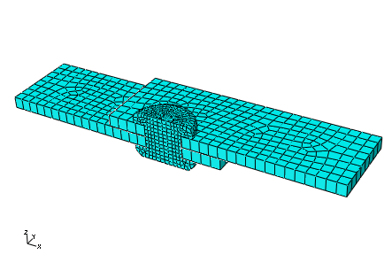
The model consists of two overlapping aluminum plates that are connected with a titanium rivet. The left end of the bottom plate is fixed, and the force is applied to the right end of the top plate to shear the joint. Figure 12–31 shows the basic arrangement of the components. Because of symmetry, only half of the joint is modeled to reduce computational cost. Frictional contact is assumed.
Use Abaqus/CAE to create the model. Abaqus provides scripts that replicate the complete analysis model for this problem. Run one of these scripts if you encounter difficulties following the instructions given below or if you wish to check your work. Scripts are available in the following locations:
A Python script for this example is provided in “Shearing of a lap joint,” Section A.13 of Getting Started with Abaqus/CAE. Instructions on how to fetch the script and run it within Abaqus/CAE are given in Appendix A, “Example Files.”
A plug-in script for this example is available in the Abaqus/CAE Plug-in toolset. To run the script from Abaqus/CAE, select Plug-ins![]() Abaqus
Abaqus![]() Getting Started, highlight Lap joint, and click Run. For more information about the Getting Started plug-ins, see “Running the Getting Started with Abaqus examples,” Section 82.1 of the Abaqus/CAE User's Guide.
Getting Started, highlight Lap joint, and click Run. For more information about the Getting Started plug-ins, see “Running the Getting Started with Abaqus examples,” Section 82.1 of the Abaqus/CAE User's Guide.
Part definition
Start Abaqus/CAE (if you are not already running it). You will have to create two parts: one representing the plate and one representing the rivet.
Plate
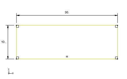
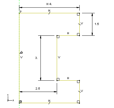
Create a three-dimensional, deformable solid part with an extruded base feature to represent the plate. Use an approximate part size of 100.0, and name the part plate. Begin by sketching a rectangle of arbitrary dimensions. Then, dimension it so that the horizontal length is 30 and the vertical length is 10, as shown in Figure 12–32.
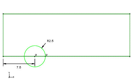
Extrude the part a distance of 1.5.Use the Create Cut: Extrude tool to cut out the circular region corresponding to the bolt hole. Select the front face of the plate as the sketch plane and the right edge of the face as the edge that will appear vertical and on the right in the sketch. Sketch the bolt hole as shown in Figure 12–33.
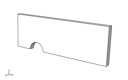
Extrude the cut through the entire part.The final shape of the plate appears as shown in Figure 12–34.
Rivet
Create a three-dimensional, deformable solid part with a revolved base feature to represent the rivet. Use an approximate part size of 20.0, and name the part rivet. Using the Create Lines tool, create a rough sketch of the rivet geometry, as shown in Figure 12–35. Use dimensions and equal length constraints as necessary to refine the sketch, as shown in Figure 12–35. Revolve the part 180 degrees.
Edit the base part to include a fillet at the top outer edge and a chamfer at the bottom outer edge. Use a radius of 0.75 for the fillet and a length of 0.75 for the chamfer. The final part geometry is shown in Figure 12–36.
Material and section properties
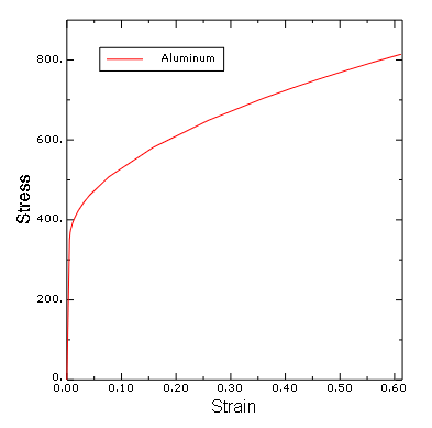
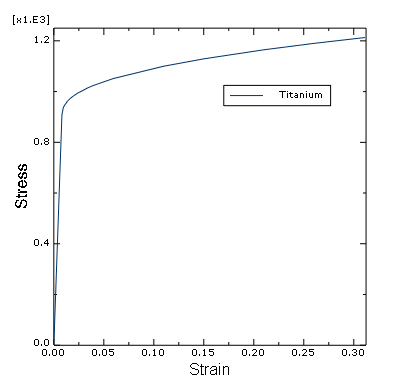
The plates are made from aluminum; the stress-strain behavior is shown in Figure 12–37. The rivet is made from titanium; the stress-strain behavior is shown in Figure 12–38.
The stress-strain data for the aluminum and titanium materials are provided in text files named lap-joint-alum.txt and lap-joint-titanium.txt, respectively. Enter the following command at the operating system prompt to use the Abaqus fetch utility to copy these files to your local directory:
abaqus fetch job=lap*.txtRather than convert the stress-strain data and define the material properties manually, you will use the material calibration capability to define the material properties.
To calibrate a material:
In the Model Tree, double-click Calibrations.
Name the calibration aluminum, and click OK.
Expand the Calibrations container and then expand the aluminum item.
Double-click Data Sets.
In the Create Data Set dialog box, enter Al as the name and click Import Data Set.
In the Read Data From Text File dialog box, click ![]() and choose the file named lap-joint-alum.txt.
and choose the file named lap-joint-alum.txt.
In the Properties region of this dialog box, specify that strain values will be read from field 2 and stress values from field 1.
From the Data Set Form options, select True to indicate that the data you are importing are in true form.
Click OK to close the Read Data From Text File dialog box.
Click OK to close the Create Data Set dialog box.
In the Model Tree, double-click Behaviors.
Name the behavior Al-elastic-plastic, choose Elastic Plastic Isotropic as the type, and click Continue.
In the Edit Behavior dialog box, choose Al as the data set for the elastic-plastic data.
Enter 0.00488, 350.0 in the text field to define the yield point (alternatively, you could select the point directly in the viewport).
Drag the Plastic points slider midway between Min and Max to generate plastic data points.
Enter a Poisson's ratio of 0.33.
At the bottom of the dialog box, click ![]() to create an empty material named aluminum (simply click OK in the material editor after entering the name).
to create an empty material named aluminum (simply click OK in the material editor after entering the name).
In the Edit Behavior dialog box, choose aluminum from the Material drop-down list.
Click OK to add the properties to the material named aluminum.
In the Model Tree, expand the Materials container and examine the contents of the material model. You will note that both elastic and plastic properties have been defined. If you wish to change the number of plastic points or modify the yield point, simply return to the Edit Behavior dialog box, make the necessary changes, select the name of the material to which the properties will be applied, and click OK. The contents of the material model are updated automatically.
Following the same procedure, create a material model named titanium. The file containing the stress-strain data is named lap-joint-titanium.txt; the yield point is 0.0081, 907.0; and Poisson's ratio is equal to 0.34.
Create a homogeneous solid section named plate that refers to the material aluminum. Assign the section to the plate.
Create a homogeneous solid section named rivet that refers to the material titanium. Assign the section to the rivet.
Assembling the parts
You will now create an assembly of part instances to define the analysis model. The assembly consists of two dependent instances of the plate and a single dependent instance of the rivet. The first plate instance is the top plate of the assembly; the second plate instance is the bottom plate of the assembly.
To instance and position the plates:
In the Model Tree, double-click Instances underneath the Assembly container and select plate as the part to instance.
Create a second instance of the plate. Toggle on the option to automatically offset the part instances.
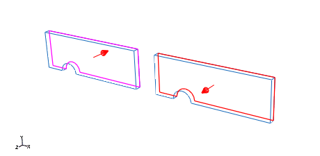
From the main menu bar, select Constraint![]() Face to Face. Select the back face of the plate on the right (the second instance) as the face on the movable instance. Select the back face of the plate on the left (the first instance) as the face on the fixed instance. If necessary, flip the arrows so that they point in opposite directions, as shown in Figure 12–39. Set the offset equal to 0.0.
Face to Face. Select the back face of the plate on the right (the second instance) as the face on the movable instance. Select the back face of the plate on the left (the first instance) as the face on the fixed instance. If necessary, flip the arrows so that they point in opposite directions, as shown in Figure 12–39. Set the offset equal to 0.0.
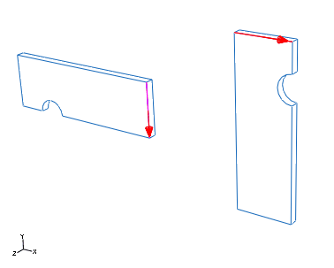
From the main menu bar, select Constraint![]() Parallel Edge. Select the front top edge of the second plate instance as the edge on the movable instance. Select the front right edge of the first plate instance as the edge on the fixed instance. If necessary, flip the arrows so that they point in the directions shown in Figure 12–40.
Parallel Edge. Select the front top edge of the second plate instance as the edge on the movable instance. Select the front right edge of the first plate instance as the edge on the fixed instance. If necessary, flip the arrows so that they point in the directions shown in Figure 12–40.
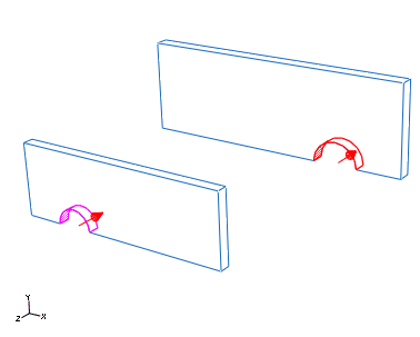
From the main menu bar, select Constraint![]() Coaxial. Select the cylindrical face of the second plate instance as the face on the movable instance. Select the cylindrical face of the first plate instance as the face on the fixed instance. If necessary, flip the arrows so that they point in the same direction, as shown in Figure 12–41.
Coaxial. Select the cylindrical face of the second plate instance as the face on the movable instance. Select the cylindrical face of the first plate instance as the face on the fixed instance. If necessary, flip the arrows so that they point in the same direction, as shown in Figure 12–41.
To instance and position the rivet:
In the Model Tree, double-click Instances underneath the Assembly container and select rivet as the part to instance.
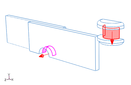
From the main menu bar, select Constraint![]() Coaxial. Select the cylindrical face of the rivet body as the face on the movable instance. Select the cylindrical face of the top plate as the face on the fixed instance. Flip the arrows if necessary so that they point in the directions shown in Figure 12–42.
Coaxial. Select the cylindrical face of the rivet body as the face on the movable instance. Select the cylindrical face of the top plate as the face on the fixed instance. Flip the arrows if necessary so that they point in the directions shown in Figure 12–42.
The final assembly is shown in Figure 12–31.
Geometry sets
At this point it is convenient to create the geometry sets that will be used to specify loads and boundary conditions.
To create geometry sets:
Double-click the Sets item underneath the Assembly container to create the following geometry sets:
corner at the lower left vertex of the bottom plate (Figure 12–43). This set will be used to prevent rigid body motion in the 3-direction.
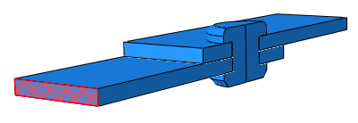
fix at the left face of the bottom plate (Figure 12–44). This set will be used to fix the end of the plate.
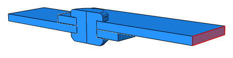
pull at the right face of the top plate (Figure 12–45). This set will be used to pull the end of the plate.
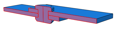
symm to include all faces on the symmetry plane (Figure 12–46). This set will be used to impose symmetry conditions.
Defining steps and output requests
Create a single static, general step after the Initial step, and include the effects of geometric nonlinearity. Set the initial time increment to 0.05 and the total time to 1.0. Accept the default output requests.
Defining contact interactions
Contact will be used to enforce the interactions between the plates and the rivet. The friction coefficient between all parts is assumed to be 0.05.
This problem could use either contact pairs or the general contact algorithm. We will use general contact in this problem to demonstrate the simplicity of the user interface.
Define a contact interaction property named fric. In the Edit Contact Property dialog box, select Mechanical![]() Tangential Behavior, select Penalty as the friction formulation, and specify a friction coefficient of 0.05 in the table. Accept all other defaults.
Tangential Behavior, select Penalty as the friction formulation, and specify a friction coefficient of 0.05 in the table. Accept all other defaults.
Create a General contact (Standard) interaction named All in the Initial step. In the Edit Interaction dialog box, accept the default selection of All* with self for the Contact Domain to specify self-contact for the default unnamed, all-inclusive surface defined automatically by Abaqus/Standard. This method is the simplest way to define contact in Abaqus/Standard for an entire model. Select fric as the Global property assignment, and click OK.
Defining boundary conditions
The boundary conditions are defined in the static, general step. The left end of the assembly is fixed while the right end is pulled along the length of the plates (1-direction). A single node is fixed in the vertical (3-) direction to prevent rigid body motion, while the nodes on the symmetry plane are fixed in the direction normal to the plane (2-direction). The boundary conditions are summarized in Table 12–3. Define these conditions in the model.
Mesh creation and job definition
The mesh will be created at the part level rather than the assembly level, since all part instances used in this problem are dependent. The dependent instances will inherit the part mesh. Begin by expanding the container for the part named plate in the Model Tree, and double-click Mesh to switch to the Mesh module.
Mesh the plate with C3D8I elements using a global seed size of 1.2 and the default sweep mesh technique.
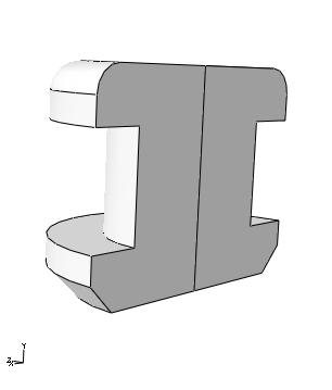
Similarly, mesh the rivet with C3D8R elements using a global seed size of 0.5 and the hex-dominated sweep mesh technique. This mesh technique will create wedge-shaped elements (C3D6) about the rivet’s axis of symmetry. The meshed assembly appears in Figure 12–47.
Note: If you are using the Abaqus Student Edition, these seed sizes will result in a mesh that exceeds the model size limits of the product. For the plate specify a global seed size of 1.75, with a maximum curvature deviation factor of 0.05. For the rivet specify a global seed size of 1.
You are now ready to create and run the job. Create a job named lap_joint. Save your model to a model database file, and submit the job for analysis. Monitor the solution progress, correct any modeling errors that are detected, and investigate the cause of any warning messages.
In the Visualization module, examine the deformation of the assembly.
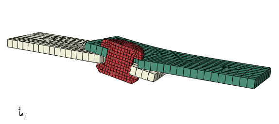
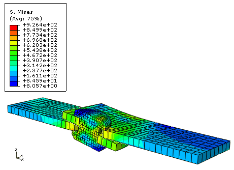
Deformed model shape and contour plots
The basic results of this simulation are the deformation of the joint and the stresses caused by the shearing process. Plot the deformed model shape and the Mises stress, as shown in Figure 12–48 and Figure 12–49, respectively.
Contact pressures
You will now plot the contact pressures in the lap joint.
Since it is difficult to see contact pressures when the entire model is displayed, use the Display Groups toolbar to display only the top plate in the viewport.
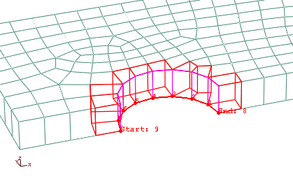
Create a path plot to examine the variation of the contact pressure around the bolt hole of the top plate.
To create a path plot:
In the Results Tree, double-click Paths. In the Create Path dialog box, select Edge list as the type and click Continue.
In the Edit Edge List Path dialog box, select the instance corresponding to the top plate and click Add After.
In the prompt area, select by shortest distance as the selection method.
In the viewport, select the edge at the left end of the bolt hole as the starting edge of the path and the node at the right end of the bolt hole as the end node of the path, as shown in Figure 12–50.
Click Done in the prompt area to indicate that you have finished making selections for the path. Click OK to save the path definition and to close the Edit Edge List Path dialog box.
In the Results Tree, double-click XYData. Select Path in the Create XY Data dialog box, and click Continue.
In the Y Values frame of the XY Data from Path dialog box, click Step/Frame. In the Step/Frame dialog box, select the last frame of the step. Click OK to close the Step/Frame dialog box.
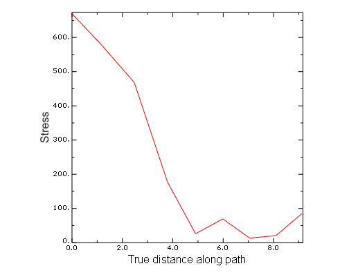
Make sure that the field output variable is set to CPRESS, and click Plot to view the path plot. Click Save As to save the plot.
The path plot appears as shown in Figure 12–51.