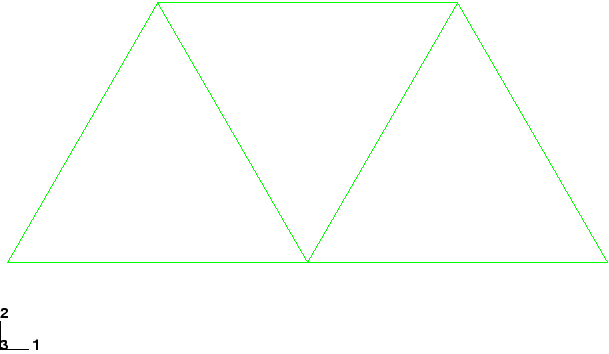
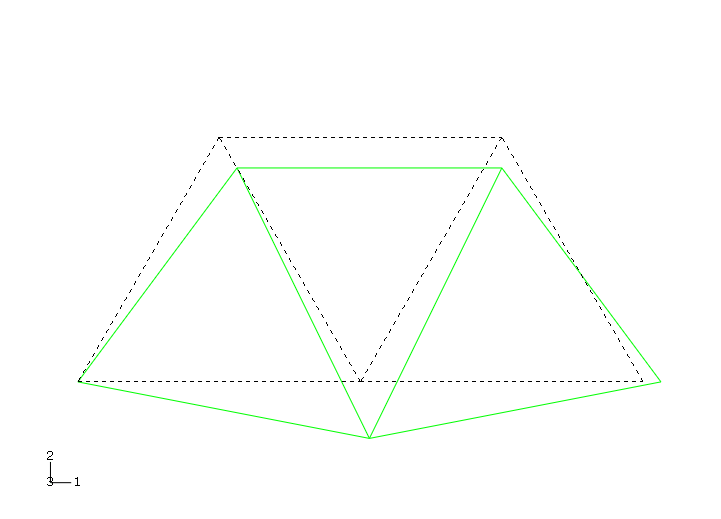
The simulation of the pin-jointed, overhead hoist in Figure 2–1 is used to illustrate the creation of an Abaqus input file using an editor. As you read through this section, you should type the data into a file using one of the editors available on your computer. The Abaqus input file must have an .inp file extension. For convenience, name the input file frame.inp. The file identifier, which can be chosen to identify the analysis, is called the jobname. In this case use the jobname “frame” to associate it easily with the input file called frame.inp.
All of the other examples in this guide assume that you will be using a preprocessor, such as Abaqus/CAE, to generate the mesh if you are going to create the model from scratch. Input files for all the examples are available. See Appendix A, “Example Files,” for instructions on how to retrieve these input files. However, since the purpose of this example is to help you understand the structure and format of the Abaqus input file, you should type this input file in directly, rather than use a preprocessor or copy the input file that is provided. If you wish to create the entire model using Abaqus/CAE, refer to “Example: creating a model of an overhead hoist,” Section 2.3 of Getting Started with Abaqus: Interactive Edition.
Before starting to define this or any model, you need to decide which system of units you will use. Abaqus has no built-in system of units. Do not include unit names or labels when entering data in Abaqus. All input data must be specified in consistent units. Some common systems of consistent units are shown in Table 2–1.
| Quantity | SI | SI (mm) | US Unit (ft) | US Unit (inch) |
|---|---|---|---|---|
| Length | m | mm | ft | in |
| Force | N | N | lbf | lbf |
| Mass | kg | tonne (103 kg) | slug | lbf s2/in |
| Time | s | s | s | s |
| Stress | Pa (N/m2) | MPa (N/mm2) | lbf/ft2 | psi (lbf/in2) |
| Energy | J | mJ (103 J) | ft lbf | in lbf |
| Density | kg/m3 | tonne/mm3 | slug/ft3 | lbf s2/in4 |
The SI system of units is used throughout this guide. Users working in the systems labeled “US Unit” should be careful with the units of density; often the densities given in handbooks of material properties are multiplied by the acceleration due to gravity.
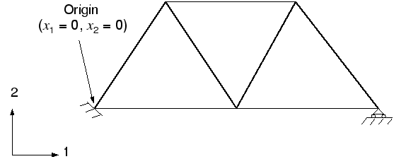
You also need to decide which coordinate system to use. The global coordinate system in Abaqus is a right-handed, rectangular (Cartesian) system. For this example define the global 1-axis to be the horizontal axis of the hoist and the global 2-axis to be the vertical axis (Figure 2–3). The global 3-axis is normal to the plane of the framework. The origin (![]() =0,
=0, ![]() =0,
=0, ![]() =0) is the bottom left-hand corner of the frame.
=0) is the bottom left-hand corner of the frame.
For two-dimensional problems, such as this one, Abaqus requires that the model lie in a plane parallel to the global 1–2 plane.
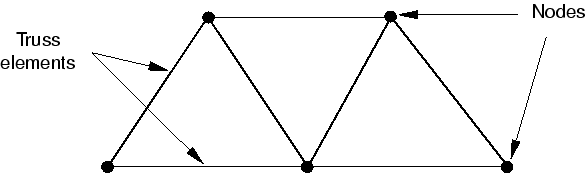
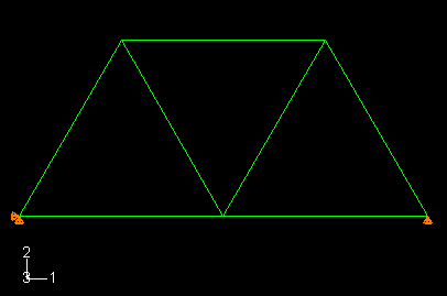
You must select the element types and design the mesh. Creating a proper mesh for a given problem requires experience. For this example you will use a single truss element to model each member of the frame, as shown in Figure 2–4.
A truss element, which can carry only tensile and compressive axial loads, is ideal for modeling pin-jointed frameworks, such as the overhead hoist. Truss elements are described in “Truss elements,” Section 3.1.5, and also in the Abaqus Analysis User's Guide, which describes every element available in Abaqus. The index of element types (Section EI.1, “Abaqus/Standard Element Index,” of the Abaqus Analysis User's Guide) makes locating a particular element easy. Whenever you are using an element for the first time, you should read the description, which includes the element connectivity and any element section properties needed to define the element's geometry.
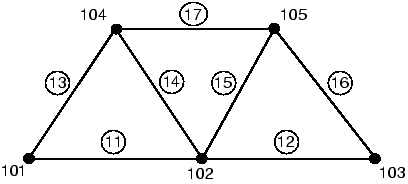
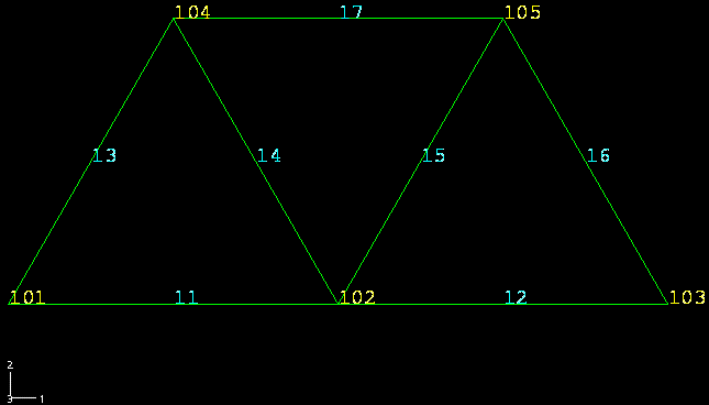
The connectivity for the truss elements used in the overhead hoist model is shown in Figure 2–5.
Node and element numbers are merely identification labels. They are usually generated automatically by Abaqus/CAE or another preprocessor. The only requirement for node and element numbers is that they must be positive integers. Gaps in the numbering are allowed, and the order in which nodes and elements are defined does not matter. Any nodes that are defined but not associated with an element are removed automatically and are not included in the simulation.
In this case we use the node and element numbers shown in Figure 2–6.
The first part of the input file must contain all of the model data. These data define the structure being analyzed. In the overhead hoist example the model data consist of the following:
Geometry:
Nodal coordinates.
Element connectivity.
Element section properties.
Material properties.
Heading
The first option in any Abaqus input file must be *HEADING. The data lines that follow the *HEADING option are lines of text describing the problem being simulated. You should provide an accurate description to allow the input file to be identified at a later date. Moreover, it is often helpful to specify the system of units, directions of the global coordinate system, etc. For example, the *HEADING option block for the hoist problem contains the following:
*HEADING
Two-dimensional overhead hoist frame
SI units (kg, m, s, N)
1-axis horizontal, 2-axis vertical
Data file printing options
By default, Abaqus will not print an echo of the input file or the model and history definition data to the printed output (.dat) file. However, it is recommended that you check your model and history definition in a datacheck run before performing the analysis. The datacheck run is discussed later in this chapter.
To request a printout of the input file and of the model and history definition data, add the following statement to the input file:
*PREPRINT, ECHO=YES, MODEL=YES, HISTORY=YES
Nodal coordinates
The coordinates of each node can be defined once you select the mesh design and node numbering scheme. For this problem use the numbering shown in Figure 2–6. The coordinates of nodes are defined using the *NODE option. Each data line of this option block has the form
<node number>,<The nodes for the hoist model are defined as follows:-coordinate>,<
-coordinate>,<
-coordinate>
*NODE
101, 0.,  0.,    0.
102, 1.,  0.,    0.
103, 2.,  0.,    0.
104, 0.5, 0.866, 0.
105, 1.5, 0.866, 0.
Element connectivity
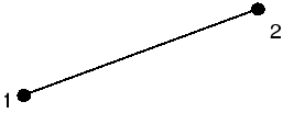
The members of the overhead hoist are modeled with truss elements. The format of each data line for a truss element is
<element number>, <node 1>, <node 2>where node 1 and node 2 are at the ends of the element (see Figure 2–5). For example, element 16 connects nodes 103 and 105 (see Figure 2–6), so the data line defining this element is
16, 103, 105The TYPE parameter on the *ELEMENT option must be used to specify the kind of element being defined. In this case you will use T2D2 truss elements.
One of the most useful features in Abaqus is the availability of node and element sets that are referred to by name. By using the ELSET parameter on the *ELEMENT option, all of the elements defined in the option block are added to an element set called FRAME. A set name can have as many as 80 characters and must start with a letter. Since element section properties are assigned through element set names, all elements in the model must belong to at least one element set.
The complete *ELEMENT option block for the overhead hoist model (see Figure 2–6) is shown below:
*ELEMENT, TYPE=T2D2, ELSET=FRAME
11, 101, 102
12, 102, 103
13, 101, 104
14, 102, 104
15, 102, 105
16, 103, 105
17, 104, 105
Element section properties
Each element must refer to an element section property. The appropriate element section option for each element and the additional geometric data (if any) needed for each element are described in the Abaqus Analysis User's Guide.
For the T2D2 element you must use the *SOLID SECTION option and give one data line with the cross-sectional area of the element. If you leave the data line blank, the cross-sectional area is assumed to be 1.0.
In this case all the members are circular bars that are 5 mm in diameter. Their cross-sectional area is 1.963 × 10⁵ m2.
The MATERIAL parameter, which is required for most element section options, refers to the name of a material property definition that is to be used with the elements. The name can have up to 80 characters and must begin with a letter.
In this example all of the elements have the same section properties and are made of the same material. Typically, there will be several different element section properties in an analysis; for example, different components in a model may be made of different materials. The elements are associated with material properties through element sets. For the overhead hoist model the elements are added to an element set called FRAME. Element set FRAME is then used as the value of the ELSET parameter on the element section option. Add the following option block to your input file:

Materials
One of the features that makes Abaqus a truly general-purpose finite element program is that almost any material model can be used with any element. Once the mesh has been created, material models can be associated, as appropriate, with the elements in the mesh.
Abaqus has a large number of material models, many of which include nonlinear behavior. In this overhead hoist example we use the simplest form of material behavior: linear elasticity. In Chapter 10, “Materials,” two of the most common forms of nonlinear material behavior are considered: metal plasticity and rubber elasticity. A discussion of all the material models available in Abaqus can be found in the Abaqus Analysis User's Guide.
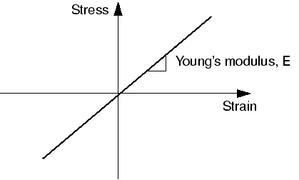
Linear elasticity is appropriate for many materials at small strains, particularly for metals up to their yield point. It is characterized by a linear relationship between stress and strain (Hooke's law), as shown in Figure 2–7.
The material behavior is characterized by two constants: Young's modulus, E, and Poisson's ratio, ![]() .
.
A material definition in the Abaqus input file starts with a *MATERIAL option. The parameter NAME is used to associate a material with an element section property. For example,
*SOLID SECTION, ELSET=FRAME, MATERIAL=STEEL
1.963E-5
*MATERIAL, NAME=STEEL
Material suboptions directly follow their associated *MATERIAL option. Several suboptions may be required to complete the material definition. All material suboptions are associated with the material that is listed on the most recent *MATERIAL option until another *MATERIAL option or a non-material option block is given.
Without considering thermal expansion effects (which would be defined with the *EXPANSION material suboption), one material suboption, *ELASTIC, is required to define a linear elastic material. The form of this option block is
*ELASTIC <E>,<Therefore, the complete, isotropic, linear elastic material definition for the hoist members, which are made of steel, should be entered into your input file as>
*MATERIAL, NAME=STEEL
*ELASTIC
200.E9, 0.3
The model definition portion of this problem is now complete since all the components describing the structure have been specified.
The history data define the sequence of events for the simulation. This loading history is divided into a series of steps, each defining a different portion of the structure's loading. Each step contains the following information:
the type of simulation (static, dynamic, etc.);
the loads and constraints; and
the output required.
In this example we are interested in the static response of the overhead hoist to a 10 kN load applied at the midspan, with the left-hand end fully constrained and a roller constraint on the right-hand end (see Figure 2–1). This is a single event, so only a single step is needed for the simulation.
The *STEP option is used to mark the start of a step. Like the *HEADING option, this option may be followed by data lines containing a title for the step. In your hoist model use the following *STEP option block:
*STEP, PERTURBATION
10kN central load
The PERTURBATION parameter indicates that this is a linear analysis. If this parameter is omitted, the analysis may be linear or nonlinear. The use of the PERTURBATION parameter is discussed further in Chapter 11, “Multiple Step Analysis.”
Analysis procedure
The analysis procedure (the type of simulation) must be defined immediately following the *STEP option block. In this case we want the long-term static response of the structure. The option for a static simulation is *STATIC. For linear analysis this option has no parameters or data lines, so add the following line to your input file:
*STATIC
The remaining input data in the step define the boundary conditions (constraints), loads, and output required and can be given in any order that is convenient.
Boundary conditions
Boundary conditions are applied to those parts of the model where the displacements are known. Such parts may be constrained to remain fixed (have zero displacement) during the simulation or may have specified, nonzero displacements. In either situation the constraints are applied directly to the nodes of the model.
In some cases a node may be constrained completely and, thus, cannot move in any direction (for example, node 101 in our case). In other cases a node is constrained in some directions but is free to move in others. For example, node 103 is fixed in the vertical direction but is free to move in the horizontal direction. The directions in which a node is able to move are called degrees of freedom (dof). In the case of our two-dimensional hoist, each node can move in the global 1- and 2-directions; therefore, there are two degrees of freedom at each node. If the hoist could move out of plane, the problem would be three-dimensional, and each node would have three degrees of freedom. Nodes attached to beam and shell elements have additional degrees of freedom representing the components of rotation and, thus, may have up to six degrees of freedom.
The labeling convention used for the degrees of freedom in Abaqus is as follows:
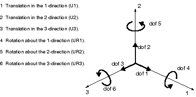
The degrees of freedom active at a node depend on the type of elements attached to that node. Chapter 3, “Finite Elements and Rigid Bodies,” describes the active degrees of freedom for some of the elements available in Abaqus. The two-dimensional truss element, T2D2, has two degrees of freedom active at each node—translation in the 1- and 2-directions (dof 1 and dof 2, respectively).
Constraints on nodes are defined by using the *BOUNDARY option and specifying the constrained degrees of freedom. Each data line is of the form:
<node number>, <first dof>, <last dof>, <magnitude of displacement>
The first degree of freedom and last degree of freedom are used to give a range of degrees of freedom that will be constrained. For example, the following statement constrains degrees of freedom 1, 2, and 3 at node 101 to have zero displacement (the node cannot move in either the global 1-, 2-, or 3-direction):
101, 1, 3, 0.0
If the magnitude of the displacement is not specified on the data line, it is assumed to be zero. If the node is constrained in one direction only, the third field should be blank or equal to the second field. For example, to constrain node 103 in the 2-direction (degree of freedom 2) only, any of the following data line formats can be used:
103, 2,2, 0.0or
103, 2,2or
103, 2
Boundary conditions on a node are cumulative. Thus, the following input constrains node 101 in both directions 1 and 2:
101, 1
101, 2
Rather than specifying each constrained degree of freedom, some of the more common constraints can be given directly using the following named constraints:
| Degree of freedom | Description |
|---|---|
| ENCASTRE | Constraint on all displacements and rotations at a node. |
| PINNED | Constraint on all translational degrees of freedom. |
| XSYMM | Symmetry constraint about a plane of constant |
| YSYMM | Symmetry constraint about a plane of constant |
| ZSYMM | Symmetry constraint about a plane of constant |
| XASYMM | Antisymmetry constraint about a plane of constant |
| YASYMM | Antisymmetry constraint about a plane of constant |
| ZASYMM | Antisymmetry constraint about a plane of constant |
101, ENCASTRE
The complete *BOUNDARY option block for our hoist problem is:
*BOUNDARY
101, ENCASTRE
103, 2
In this example all of the constraints are in the global 1- or 2-directions. In many cases constraints are required in directions that are not aligned with the global directions. The *TRANSFORM option can be used in such cases to define a local coordinate system for boundary condition application. The skew plate example in Chapter 5, “Using Shell Elements,” demonstrates how to use this option in such cases.
Loading
Loading is anything that causes the displacement or deformation of the structure, including:
concentrated loads,
pressure loads,
distributed traction loads,
distributed edge loads and moment on shells,
nonzero boundary conditions,
body loads, and
temperature (with thermal expansion of the material defined).
In reality there is no such thing as a concentrated, or point, load; the load will always be applied over some finite area. However, if the area being loaded is similar to or smaller than the elements in that area, it is an appropriate idealization to treat the load as a concentrated load applied to a node.
Concentrated loads are specified using the *CLOAD option. The data lines for this option have the form:
<node number>, <dof>, <load magnitude>In this simulation a load of 10 kN is applied in the 2-direction to node 102. The option block is:
*CLOAD
102, 2, -10.E3
Output requests
Finite element analyses can create very large amounts of output. Abaqus allows you to control and manage this output so that only data required to interpret the results of your simulation are produced. Four types of output are available:
Results stored in a neutral binary file used by Abaqus/Viewer for postprocessing. This file is called the Abaqus output database file and has the extension .odb.
Printed tables of results, written to the Abaqus data (.dat) file.
Restart data, used to continue the analysis, written to the Abaqus restart (.res) file.
Results stored in binary files for subsequent postprocessing with third-party software, written to the Abaqus results (.fil) file.
By default, an output database file, which includes a preselected set of the most commonly used output variables for a given type of analysis, is created. A list of preselected variables for default output database output is given in the Abaqus Analysis User's Guide. You do not need to add any output requests to accept these defaults. For this example the default output database output includes the deformed configuration and the applied nodal loads.
Selected results also can be written in tabular form to the Abaqus data file. By default, no printout is written to the Abaqus data file. The *NODE PRINT option controls the printing of nodal results (for example, displacements and reaction forces), while the *EL PRINT option controls the printing of element results. A comprehensive list of the output variables available is given in the Abaqus Analysis User's Guide.
The data lines for either of these options list the output to appear in the columns of the table. Each data line creates a separate table of data that can have a maximum of nine columns.
For this analysis we are interested in the displacements of the nodes (output variable U), the reaction forces at the constrained nodes (output variable RF), and the stress in the members (output variable S). Use the following in your input file:
*NODE PRINT
U,
RF,
*EL PRINT
S,
to request that Abaqus generate three tables of output data in the data file.
Since you have now finished the definition of all the data required for the step, use the *END STEP option to mark the end of the step:
*END STEP
The input file is now complete. Compare the input file you have generated to the complete input file given in Figure 2–2. Save the data as frame.inp, and exit the editor.
Having generated the input file for this simulation, you are ready to run the analysis. Unfortunately, it is possible to have errors in the input file because of typing errors or incorrect or missing data. You should perform a datacheck analysis first before running the simulation. To run a datacheck analysis, make sure that you are in the directory where the input file frame.inp is located, and type the following command:
abaqus job=frame datacheck interactive
If this command results in an error message, the Abaqus installation on your computer has been customized. You should contact your systems administrator to find out the appropriate command to run Abaqus. The job=frame parameter specifies that the jobname for this analysis is frame. All the files associated with this analysis will have this jobname as their identifier, which allows them to be recognized easily.
The analysis will run interactively, and messages similar to those shown below will appear on your screen:
Abaqus JOB frame
Abaqus 6.14-1
Begin Analysis Input File Processor
9/23/2010 9:26:43 AM
Run pre.exe
Abaqus License Manager checked out the following licenses:
Abaqus/Foundation checked out 3 tokens.
9/23/2010 9:26:45 AM
End Analysis Input File Processor
Begin Abaqus/Standard Datacheck
Begin Abaqus/Standard Analysis
9/23/2010 9:26:45 AM
Run standard.exe
Abaqus License Manager checked out the following licenses:
Abaqus/Foundation checked out 3 tokens.
2/23/2010 9:26:45 AM
End Abaqus/Standard Analysis
Abaqus JOB frame COMPLETED
When the datacheck analysis is complete, you will find that a number of additional files have been created by Abaqus. If any errors are encountered during the datacheck analysis, messages will be written to the data file, frame.dat. This data file is a text file that can be viewed in an editor or printed. Try viewing the data file in a text editor. The file can contain lines up to 256 characters long, so the editor should be able to accommodate that many characters.
Header page
The data file starts with a header page that contains information about the release of Abaqus used to run the analysis. The header page also contains the phone number, address, and contact information of your local office or representative who can offer technical support and advice.
Input file echo
After the header page, the data file includes an echo of the input file. The input data echo is generated by adding the option *PREPRINT, ECHO=YES to the input file. By default, the parameter ECHO is set to NO.
                                         A B A Q U S   I N P U T   E C H O


                   5   10   15   20   25   30   35   40   45   50   55   60   65   70   75   80
               --------------------------------------------------------------------------------
               *HEADING
               Two-dimensional overhead hoist frame
               SI units (kg, m, s, N)
               1-axis horizontal, 2-axis vertical
LINE     5     *PREPRINT, ECHO=YES, MODEL=YES, HISTORY=YES
               **
               ** Model definition
               **
               *NODE, NSET=NALL
LINE    10     101, 0.,  0.,    0.
               102, 1.,  0.,    0.
               103, 2.,  0.,    0.
               104, 0.5, 0.866, 0.
               105, 1.5, 0.866, 0.
LINE    15     *ELEMENT, TYPE=T2D2, ELSET=FRAME
               11, 101, 102
               12, 102, 103
               13, 101, 104
               14, 102, 104
LINE    20     15, 102, 105
               16, 103, 105
               17, 104, 105
               *SOLID SECTION, ELSET=FRAME, MATERIAL=STEEL
               ** diameter = 5mm --> area = 1.963E-5 m^2
LINE    25     1.963E-5,
               *MATERIAL, NAME=STEEL
               *ELASTIC
               200.E9, 0.3
               **
LINE    30     ** History data
               **
               *STEP, PERTURBATION
               10kN central load
               *STATIC
LINE    35     *BOUNDARY
               101, ENCASTRE
               103, 2
               *CLOAD
               102, 2, -10.E3
LINE    40     *NODE PRINT
               U,
               RF,
               *EL PRINT
               S,
LINE    45     *END STEP
               --------------------------------------------------------------------------------
                   5   10   15   20   25   30   35   40   45   50   55   60   65   70   75   80
               --------------------------------------------------------------------------------
Options processed by Abaqus
Following the input data echo is a list of the options processed by Abaqus. This is the first point at which error and warning messages appear. All error messages are prefixed with ***ERROR, while warnings begin with ***WARNING. Since these messages always begin the same way, searching the data file for warning and error messages is straightforward. When the error is a syntax problem (i.e., when Abaqus cannot understand the input), the error message is followed by the line from the input file that is causing the error.
OPTIONS BEING PROCESSED
***************************


*HEADING
        Two-dimensional overhead hoist frame
*NODE, NSET=NALL
*ELEMENT, TYPE=T2D2, ELSET=FRAME
*MATERIAL, NAME=STEEL
*ELASTIC
*SOLID SECTION, ELSET=FRAME, MATERIAL=STEEL
*BOUNDARY
*SOLID SECTION, ELSET=FRAME, MATERIAL=STEEL
*STEP, PERTURBATION
*STEP, PERTURBATION
*STEP, PERTURBATION
10kN central load
*STATIC
*BOUNDARY
*EL PRINT
*EL FILE
*END STEP
*STEP, PERTURBATION
*STATIC
*BOUNDARY
*CLOAD
*NODE PRINT
*NODE FILE
*END STEP
Model data
The rest of the data file is a series of tables containing all of the model data and the history data that should be checked for any obvious errors or omissions. These tables are generated by including the option *PREPRINT, MODEL=YES, HISTORY=YES in the input file. However, these tables may take up a large amount of disk space for large models. By default, the parameters MODEL and HISTORY are set to NO.
The model data section begins with the element definitions, which summarize all the model data. The model data also include the material description. It is always a good idea to check that Abaqus has interpreted the material properties you gave in the input file correctly. Mistakes in the material properties can sometimes cause subtle errors that are difficult to detect from the results. It is easier to check the data here.
      E L E M E N T   D E F I N I T I O N S

NUMBER   TYPE    PROPERTY    NODES FORMING ELEMENT
                 REFERENCE

  11     T2D2        1        101       102
  12     T2D2        1        102       103
  13     T2D2        1        101       104
  14     T2D2        1        102       104
  15     T2D2        1        102       105
  16     T2D2        1        103       105
  17     T2D2        1        104       105


                              S O L I D   S E C T I O N (S)


PROPERTY NUMBER         1

   MATERIAL NAME                     STEEL
   ATTRIBUTES                         1.96300E-05   0.0000       0.0000

   HOURGLASS CONTROL STIFFNESS    3.84615E+08

   (USED WITH LOWER ORDER REDUCED INTEGRATED SOLID ELEMENTS LIKE CPS4R,CPE4RH,C3D8R)


                       M A T E R I A L   D E S C R I P T I O N


MATERIAL NAME: STEEL


   ELASTIC         YOUNG'S    POISSON'S
                   MODULUS      RATIO
                  2.00000E+11 0.30000


                               E L E M E N T   S E T S


SET    FRAME
MEMBERS                  11       12       13       14       15       16       17


                                  N O D E   S E T S


SET    NALL
MEMBERS                  101       102       103       104       105


                               N O D E   D E F I N I T I O N S

     NODE           COORDINATES                       SINGLE POINT CONSTRAINTS
    NUMBER                                              TYPE    PLUS    DOF

      101     0.0000       0.0000       0.0000       ENCASTRE
      102     1.0000       0.0000       0.0000
      103     2.0000       0.0000       0.0000                    2
      104    0.50000      0.86600       0.0000
      105     1.5000      0.86600       0.0000
History data: loads and database output
The history data are presented below in two sections. The first line of the top half of the history data reads 10kN central load, which is the first data line given in the *STEP option block. This line reminds you of the loads applied in this step.
     10kN central load

     FIXED TIME INCREMENTS
     TIME INCREMENT IS                                    2.220E-16
     TIME PERIOD IS                                       2.220E-16
GLOBAL STABILIZATION CONTROL IS NOT USED

THIS IS A LINEAR PERTURBATION STEP.
ALL LOADS ARE DEFINED AS CHANGE IN LOAD TO THE REFERENCE STATE

EXTRAPOLATION WILL NOT BE USED

CHARACTERISTIC ELEMENT LENGTH      1.00

DETAILS REGARDING ACTUAL SOLUTION WAVEFRONT REQUESTED

DETAILED OUTPUT OF DIAGNOSTICS TO DATABASE REQUESTED

PRINT OF INCREMENT NUMBER, TIME, ETC., TO THE MESSAGE FILE EVERY     1  INCREMENTS


                            D A T A B A S E   O U T P U T   G R O U P       1

THE FOLLOWING  FIELD   OUTPUT WILL BE WRITTEN EVERY        1 INCREMENT(S)


THE FOLLOWING OUTPUT WILL BE WRITTEN FOR ALL ELEMENTS OF TYPE T2D2.  OUTPUT IS AT THE
INTEGRATION POINTS.

          S         E


 THE FOLLOWING OUTPUT WILL BE WRITTEN FOR ALL NODES

          U         RF        CF


END OF DATABASE OUTPUT GROUP    1


                            D A T A B A S E   O U T P U T   G R O U P       2


THE FOLLOWING HISTORY  OUTPUT WILL BE WRITTEN EVERY        1 INCREMENT(S)


THE FOLLOWING ENERGY OUTPUT QUANTITIES WILL BE WRITTEN FOR THE WHOLE MODEL

         ALLKE    ALLSE    ALLWK    ALLPD    ALLCD    ALLVD    ALLKL    ALLAE    ALLQB

         ALLEE    ALLIE    ETOTAL   ALLFD    ALLJD    ALLSD    ALLDMD

END OF DATABASE OUTPUT GROUP    2
History data: summary
The second half of the history data is displayed below. This section summarizes the element and nodal output requests, boundary conditions, and concentrated loads.
                                  E L E M E N T   P R I N T

THE FOLLOWING TABLE IS PRINTED AT EVERY 1 INCREMENT FOR ALL ELEMENTS OF TYPE T2D2.  OUTPUT IS AT
THE INTEGRATION POINTS.

  SUMMARIES WILL BE PRINTED WHERE APPLICABLE

       TABLE     1  S11


                               E L E M E N T   F I L E   O U T P U T

 THE FOLLOWING TABLE IS OUTPUT AT EVERY 1 INCREMENT FOR ALL ELEMENTS OF TYPE T2D2.  OUTPUT IS AT
 THE INTEGRATION POINTS.

          S


                                    N O D E   P R I N T

 THE FOLLOWING TABLE IS PRINTED FOR ALL NODES AT EVERY 1 INCREMENT

   SUMMARIES WILL BE PRINTED

        TABLE  1  U1        U2

 THE FOLLOWING TABLE IS PRINTED FOR ALL NODES AT EVERY 1 INCREMENT

   SUMMARIES WILL BE PRINTED

        TABLE  2  RF1       RF2


                              N O D E   F I L E   O U T P U T

THE FOLLOWING TABLE IS OUTPUT FOR ALL NODES AT EVERY 1 INCREMENT

                  U         RF


                       B O U N D A R Y   C O N D I T I O N S


NODE      DOF     AMP.    MAGNITUDE                 NODE      DOF     AMP.    MAGNITUDE
                  REF.                                                REF.

103        2     (RAMP)     0.0000

- (RAMP) OR (STEP) - INDICATE USE OF DEFAULT AMPLITUDES ASSOCIATED WITH THE STEP


                     B O U N D A R Y   C O N D I T I O N S


NODE   TYPE        NODE    TYPE        NODE    TYPE        NODE    TYPE        NODE    TYPE

101   ENCASTRE


                   C O N C E N T R A T E D   L O A D S

NODE  DOF   AMP.  AMPLITUDE     NODE  DOF   AMP.  AMPLITUDE    NODE  DOF   AMP.  AMPLITUDE
            REF.                            REF.                           REF.

102     2          -10000.
Remaining items in the data file
If there are any error messages, the number of such messages produced during the datacheck analysis is listed at the end of the data file. If there are only warning messages, the number of these messages is listed at the bottom of the data file after any of the requested output.
If error messages are generated during the datacheck analysis, it will not be possible to perform the analysis until the causes of the error messages are corrected. The causes of warning messages should always be investigated. Sometimes, warning messages are indications of mistakes in the input data; other times they are harmless and can be ignored safely.
The final section of the data file, not shown in this guide, includes a summary of the size of the numerical model and an estimate of the file sizes required for the simulation. When analyzing large models, use this output to ensure that you have enough disk space available to perform the analysis.
Make any necessary corrections to your input file. When the datacheck analysis completes with no error messages, run the analysis itself by using the command
abaqus job=frame continue interactiveMessages like those below will appear on the screen:
Abaqus JOB frame
Abaqus 6.14-1
Begin Abaqus/Standard Analysis
9/23/2010 9:30:19 AM
Run standard.exe
Abaqus License Manager checked out the following licenses:
Abaqus/Foundation checked out 3 tokens.
9/23/2010 9:30:20 AM
End Abaqus/Standard Analysis
Abaqus JOB frame COMPLETED
You should always perform a datacheck analysis before running a simulation to ensure that the input data are correct and to check that there is enough disk space and memory available to complete the analysis. However, it is possible to combine the datacheck and analysis phases of the simulation by using the command
abaqus job=frame interactive
If a simulation is expected to take a substantial amount of time, it is convenient to run it in the background by omitting the interactive parameter:
abaqus job=frame
(The above commands apply for the standard Abaqus installation on a workstation. However, Abaqus jobs may be run in batch queues on some computers. If you have any questions, ask your systems administrator how to run Abaqus on your system.)
After the analysis is completed, the data file, frame.dat, will contain the tables of results requested with the *NODE PRINT and *EL PRINT options. The tables of results follow the output from the datacheck analysis. The results from the overhead hoist simulation follow.
Element output
Two-dimensional overhead hoist frame                                STEP    1  INCREMENT    1
10kN central load                                          TIME COMPLETED IN THIS STEP   0.00


                   S T E P       1     S T A T I C   A N A L Y S I S


          10kN central load

          FIXED TIME INCREMENTS
          TIME INCREMENT IS                                    2.220E-16
          TIME PERIOD IS                                       2.220E-16

     LINEAR EQUATION SOLVER TYPE         DIRECT SPARSE

     THIS IS A LINEAR PERTURBATION STEP.
     ALL LOADS ARE DEFINED AS CHANGE IN LOAD TO THE REFERENCE STATE

                   M E M O R Y   E S T I M A T E

PROCESS      FLOATING PT       MINIMUM MEMORY        MEMORY TO
             OPERATIONS           REQUIRED          MINIMIZE I/O
            PER ITERATION         (MBYTES)           (MBYTES)

    1         2.65E+002               13                 20
NOTE:
     (1) THE ESTIMATE PRINTED IS THE MAXIMUM ESTIMATE FROM THE CURRENT STEP TO THE LAST STEP
         OF THE ANALYSIS, WITH THE UNSYMMETRIC MATRIX AND SOLVER TAKEN INTO ACCOUNT IF
         APPLICABLE. SINCE THE ESTIMATE IS BASED ON THE ACTIVE DEGREES OF FREEDOM IN THE
         FIRST ITERATION OF THE CURRENT STEP, FOR PROBLEMS WITH SUBSTANTIAL CHANGES IN ACTIVE
         DEGREES OF FREEDOM BETWEEN STEPS (OR EVEN WITHIN THE SAME STEP), THE MEMORY ESTIMATE
         MIGHT BE NOTICEABLY DIFFERENT THAN THE ACTUAL USAGE. A FEW EXAMPLES ARE: PROBLEMS
         WITH SIGNIFICANT CONTACT CHANGES, PROBLEMS WITH MODEL CHANGE, PROBLEMS WITH BOTH
         STATIC STEP AND STEADY STATE DYNAMIC PROCEDURES, WHERE THE ACOUSTIC ELEMENTS WILL
         ONLY BE ACTIVATED IN THE STEADY STATE DYNAMIC STEPS.
     (2) THE ESTIMATE FOR THE FLOATING POINT OPERATIONS ON EACH PROCESS IS BASED
         ON THE INITIAL LOAD SCHEDULING AND THIS MIGHT NOT REFLECT THE ACTUAL FLOATING
         POINT OPERATIONS COMPLETED ON EACH PROCESS. DUE TO THE DYNAMIC LOAD BALANCING SCHEME,
         THE ACTUAL LOAD BALANCE IS EXPECTED TO BE BETTER THAN THE ESTIMATE PRINTED HERE.
     (3) DEPENDING ON THE SETTING OF THE memory PARAMETER, THE DISK USAGE BY SCRATCH DATA CAN
         VARY FROM CLOSE TO ZERO TO THE ESTIMATED MEMORY TO MINIMIZE I/O.
     (4) USING RESTART, WRITE CAN GENERATE A LARGE AMOUNT OF DATA.

                                INCREMENT     1 SUMMARY


 TIME INCREMENT COMPLETED  2.220E-16,  FRACTION OF STEP COMPLETED   1.00
 STEP TIME COMPLETED       2.220E-16,  TOTAL TIME COMPLETED         0.00


                             E L E M E N T   O U T P U T


THE FOLLOWING TABLE IS PRINTED FOR ALL ELEMENTS WITH TYPE T2D2 AT THE INTEGRATION POINTS

    ELEMENT  PT FOOT-       S11
                NOTE

          11   1         1.4706E+08
          12   1         1.4706E+08
          13   1        -2.9412E+08
          14   1         2.9412E+08
          15   1         2.9412E+08
          16   1        -2.9412E+08
          17   1        -2.9412E+08

 MAXIMUM                2.9412E+08
 ELEMENT                    14

 MINIMUM               -2.9412E+08
 ELEMENT                    17
Node output
             N O D E   O U T P U T


   THE FOLLOWING TABLE IS PRINTED FOR ALL NODES

       NODE FOOT-   U1          U2
            NOTE

        102      7.3531E-04 -4.6698E-03
        103      1.4706E-03   0.000
        104      1.4706E-03 -2.5472E-03
        105       0.000     -2.5472E-03

 MAXIMUM         1.4706E-03   0.000
 AT NODE               104         101

 MINIMUM          0.000     -4.6698E-03
 AT NODE               101         102


   THE FOLLOWING TABLE IS PRINTED FOR ALL NODES

       NODE FOOT-   RF1         RF2
            NOTE

        101     -9.0949E-13   5000.
        103       0.000       5000.

 MAXIMUM          0.000       5000.
 AT NODE               102         103

 MINIMUM        -9.0949E-13   0.000
 AT NODE               101         102
Are the nodal displacements and peak stresses in the individual members reasonable for this hoist and these applied loads?
It is always a good idea to check that the results of the simulation satisfy basic physical principles. In this case check that the external forces applied to the hoist sum to zero in both the vertical and horizontal directions.
What nodes have vertical forces applied to them? What nodes have horizontal forces? Do the results from your simulation match those shown here?
Abaqus also creates several other files during a simulation. One such file—the output database file, frame.odb—can be used to visualize the results graphically using Abaqus/Viewer.
Graphical postprocessing is important because of the great volume of data created during a simulation. For any realistic model it is impractical for you to try to interpret results in the tabular form of the data file. Abaqus/Viewer allows you to view the results graphically using a variety of methods, including deformed shape plots, contour plots, vector plots, animations, and X–Y plots. All of these methods are discussed in this guide. For more information on any of the postprocessing features discussed in this guide, consult the sections on the Visualization module in the Abaqus/CAE User's Guide. For this example you will use Abaqus/Viewer to do some basic model checks and to display the deformed shape of the frame.
Start Abaqus/Viewer by typing the following command at the operating system prompt:
abaqus viewerThe Abaqus/Viewer window appears.
To begin this exercise, open the output database file that Abaqus/Standard generated during the analysis of the problem.
To open the output database file:
From the main menu bar, select File![]() Open; or use the
Open; or use the ![]() tool in the File toolbar.
tool in the File toolbar.
The Open Database dialog box appears.
From the list of available output database files, select frame.odb.
Click OK.
Tip: You can also open the output database frame.odb by typing the following command at the operating system prompt:
abaqus viewer odb=frame
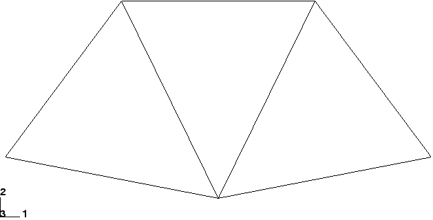
Abaqus/Viewer opens the output database created by the job and displays the undeformed model shape, as shown in Figure 2–8.
You can choose to display the title block and state block at the bottom of the viewport; these blocks are not shown in Figure 2–8. The title block at the bottom of the viewport indicates the following:
The description of the model (from the job description).
The name of the output database (from the name of the analysis job).
The product name (Abaqus/Standard or Abaqus/Explicit) and release used to generate the output database.
The date the output database was last modified.
Which step is being displayed.
The increment within the step.
The step time.
You can suppress the display of and customize the title block, state block, view orientation triad, and 3D compass by selecting Viewport![]() Viewport Annotation Options from the main menu bar (for example, many of the figures in this guide do not include the title block or the compass).
Viewport Annotation Options from the main menu bar (for example, many of the figures in this guide do not include the title block or the compass).
The Results Tree
You will use the Results Tree to query the components of the model. The Results Tree allows easy access to the history output contained in an output database file for the purpose of creating X–Y plots and also to groups of elements, nodes, and surfaces based on set names, material and section assignment, etc. for the purposes of verifying the model and also controlling the viewport display.
To query the model:
All output database files that are open in a given postprocessing session are listed underneath the Output Databases container. Expand this container and then expand the container for the output database named frame.odb.
Expand the Materials container, and click the material named STEEL.
All elements are highlighted in the viewport because only one material assignment was used in this analysis.
The Results Tree will be used more extensively in later examples to illustrate the X–Y plotting capability and manipulating the display using display groups.
Customizing an undeformed shape plot
You will now use the plot options to enable the display of node and element numbering. Plot options that are common to all plot types (undeformed, deformed, contour, symbol, and material orientation) are set in a single dialog box. The contour, symbol, and material orientation plot types have additional options, each specific to the given plot type.
To display node numbers:
From the main menu bar, select Options![]() Common; or use the
Common; or use the ![]() tool in the toolbox.
tool in the toolbox.
The Common Plot Options dialog box appears.
Click the Labels tab.
Toggle on Show node labels.
Click Apply.
Abaqus/Viewer applies the change and keeps the dialog box open.
The customized undeformed plot is shown in Figure 2–9.
To display element numbers:
In the Labels tabbed page of the Common Plot Options dialog box, toggle on Show element labels.
Click OK.
Abaqus/Viewer applies the change and closes the dialog box.
The resulting plot is shown in Figure 2–10.
Remove the node and element labels before proceeding. To disable the display of node and element numbers, repeat the above procedure and, under Labels, toggle off Show node labels and Show element labels.
Displaying and customizing a deformed shape plot
You will now display the deformed model shape and use the plot options to change the deformation scale factor. You will also superimpose the undeformed model shape on the deformed model shape.
From the main menu bar, select Plot![]() Deformed Shape; or use the
Deformed Shape; or use the ![]() tool in the toolbox. Abaqus/Viewer displays the deformed model shape, as shown in Figure 2–11.
tool in the toolbox. Abaqus/Viewer displays the deformed model shape, as shown in Figure 2–11.
For small-displacement analyses (the default formulation in Abaqus/Standard) the displacements are scaled automatically to ensure that they are clearly visible. The scale factor is displayed in the state block. In this case the displacements have been scaled by a factor of 42.83.
To change the deformation scale factor:
From the main menu bar, select Options![]() Common; or use the
Common; or use the ![]() tool in the toolbox.
tool in the toolbox.
From the Common Plot Options dialog box, click the Basic tab if it is not already selected.
From the Deformation Scale Factor area, toggle on Uniform and enter 10.0 in the Value field.
Click Apply to redisplay the deformed shape.
The state block displays the new scale factor.
To return to automatic scaling of the displacements, repeat the above procedure and, in the Deformation Scale Factor field, toggle on Auto-compute.
Click OK to close the Common Plot Options dialog box.
To superimpose the undeformed model shape on the deformed model shape:
Click the Allow Multiple Plot States ![]() tool in the toolbox to allow multiple plot states in the viewport; then click the
tool in the toolbox to allow multiple plot states in the viewport; then click the ![]() tool or select Plot
tool or select Plot![]() Undeformed Shape to add the undeformed shape plot to the existing deformed plot in the viewport.
Undeformed Shape to add the undeformed shape plot to the existing deformed plot in the viewport.
By default, Abaqus/Viewer plots the deformed model shape in green and the (superimposed) undeformed model shape in a translucent white.
The plot options for the superimposed image are controlled separately from those of the primary image. From the main menu bar, select Options![]() Superimpose; or use the
Superimpose; or use the ![]() tool in the toolbox to change the edge style of the superimposed (i.e., undeformed) image.
tool in the toolbox to change the edge style of the superimposed (i.e., undeformed) image.
From the Superimpose Plot Options dialog box, click the Color & Style tab.
In the Color & Style tabbed page, select the dashed edge style.
Click OK to close the Superimpose Plot Options dialog box and to apply the change.
Checking the model with Abaqus/Viewer
You can use Abaqus/Viewer to check that the model is correct before running the simulation. You have already learned how to draw plots of the model and to display the node and element numbers. These are useful tools for checking that Abaqus is using the correct mesh.
The boundary conditions applied to the overhead hoist model can also be displayed and checked.
To display boundary conditions on the undeformed model:
Click the ![]() tool in the toolbox to disable multiple plot states in the viewport.
tool in the toolbox to disable multiple plot states in the viewport.
Display the undeformed model shape, if it is not displayed already.
From the main menu bar, select View![]() ODB Display Options.
ODB Display Options.
In the ODB Display Options dialog box, click the Entity Display tab.
Toggle on Show boundary conditions.
Click OK.
Abaqus/Viewer displays symbols to indicate the applied boundary conditions, as shown in Figure 2–13.
Tabular data reports
In addition to the graphical capabilities described above, Abaqus/Viewer allows you to write data to a text file in a tabular format. This is a convenient alternative to writing printed data to the data ( .dat) file, especially for complicated models. Output generated this way has many uses; for example, it can be used in written reports. In this problem you will generate a report containing the element stresses, nodal displacements, and reaction forces.
To generate field data reports:
From the main menu bar, select Report![]() Field Output.
Field Output.
In the Variable tabbed page of the Report Field Output dialog box, accept the default position labeled Integration Point. Click the triangle next to S: Stress components to expand the list of available variables. From this list, toggle on S11.
In the Setup tabbed page, name the report Frame.rpt. In the Data region at the bottom of the page, toggle off Column totals.
Click Apply.
The element stresses are written to the report file.
In the Variable tabbed page of the Report Field Output dialog box, change the position to Unique Nodal. Toggle off S: Stress components, and select U1 and U2 from the list of available U: Spatial displacement variables.
Click Apply.
The nodal displacements are appended to the report file.
In the Variable tabbed page of the Report Field Output dialog box, toggle off U: Spatial displacement, and select RF1 and RF2 from the list of available RF: Reaction force variables.
In the Data region at the bottom of the Setup tabbed page, toggle on Column totals.
Click OK.
The reaction forces are appended to the report file, and the Report Field Output dialog box closes.
Open the file Frame.rpt in a text editor. The contents of this file are shown below. Your node and element numbering may be different. Very small values may also be calculated differently, depending on your system.
Stress output:
Field Output Report

Source 1
---------

   ODB: frame.odb
   Step: Step-1
   Frame: Increment      1: Step Time =   2.2200E-16

Loc 1 : Integration point values from source 1

Output sorted by column "Element Label".

Field Output reported at integration points for part: PART-1-1

         Element             Int           S.S11
           Label              Pt          @Loc 1
-------------------------------------------------
              11               1     147.062E+06
              12               1     147.062E+06
              13               1    -294.118E+06
              14               1     294.118E+06
              15               1     294.118E+06
              16               1    -294.118E+06
              17               1    -294.125E+06


  Minimum                           -294.125E+06
      At Element                              17

          Int Pt                               1
  Maximum                            294.118E+06
      At Element                              15

          Int Pt                               1
Displacement output:
Field Output Report

Source 1
---------

   ODB: frame.odb
   Step: Step-1
   Frame: Increment      1: Step Time =   2.2200E-16

Loc 1 : Nodal values from source 1

Output sorted by column "Node Label".

Field Output reported at nodes for part: PART-1-1

            Node            U.U1            U.U2
           Label          @Loc 1          @Loc 1
-------------------------------------------------
             101              0.         -5.E-33
             102     735.312E-06    -4.66977E-03
             103     1.47062E-03         -5.E-33
             104     1.47062E-03    -2.54716E-03
             105     433.681E-21    -2.54716E-03


  Minimum                     0.    -4.66977E-03

         At Node             101             102
  Maximum            1.47062E-03         -5.E-33

         At Node             104             103
Reaction force output:
Field Output Report

Source 1
---------

   ODB: frame.odb
   Step: Step-1
   Frame: Increment      1: Step Time =   2.2200E-16

Loc 1 : Nodal values from source 1

Output sorted by column "Node Label".

Field Output reported at nodes for part: PART-1-1

            Node          RF.RF1          RF.RF2
           Label          @Loc 1          @Loc 1
-------------------------------------------------
             101    -909.495E-15          5.E+03
             102              0.              0.
             103              0.          5.E+03
             104              0.              0.
             105              0.              0.


  Minimum           -909.495E-15              0.
         At Node             101             105

  Maximum                     0.          5.E+03
         At Node             105             103

           Total    -909.495E-15         10.E+03
The information obtained in these tables is the same as that examined earlier when reviewing the printed results in the data (.dat) file. The advantage of using Abaqus/Viewer to generate the tabular data is that you may create it as a postprocessing operation, whereas writing it to the data (.dat) file requires you to include the appropriate option in the input file (a preprocessing operation). Thus, Abaqus/Viewer offers greater flexibility to generate tabular output.
We will rerun the same analysis in Abaqus/Explicit for comparison. This time we are interested in the dynamic response of the hoist to the same load applied suddenly at the midspan. Before continuing, save a copy of frame.inp as frame_xpl.inp. Make all subsequent changes to the frame_xpl.inp input file. You will need to replace the static step with an explicit dynamic step, modify the output requests and the material definition, and change the element library before you can resubmit the job.
Modifying the material definition
Since Abaqus/Explicit performs a dynamic analysis, a complete material definition requires that you specify the material density. For this problem assume the density is equal to 7800 kg/m3.
You can modify the material definition by adding the *DENSITY option to the material option block. The form of this option is as follows:
*DENSITY <Thus, the complete material definition for the hoist members is:>,
*MATERIAL, NAME=STEEL
*ELASTIC
200.E9, 0.3
*DENSITY
7800.,
Replacing the analysis step
The step definition must change to reflect a dynamic, explicit analysis. Locate the existing *STEP option block, which appears as follows:
*STEP, PERTURBATION
10kN central load
Replace this option block with the following one:
*STEP
10kN central load, suddenly applied
The analysis procedure (the type of simulation) must be defined immediately following the *STEP option block. In Abaqus/Explicit the three analysis options are *DYNAMIC, EXPLICIT; *DYNAMIC TEMPERATURE-DISPLACEMENT, EXPLICIT; and *ANNEAL. The *DYNAMIC TEMPERATURE-DISPLACEMENT procedure simulates the fully coupled thermal-mechanical response of a body, while the *ANNEAL procedure simulates the relaxation of stresses and plastic strains that occurs as metals are heated to a high temperature. In this simulation we want to determine the dynamic response of the structure over a period of 0.01 s. Thus, we will use *DYNAMIC, EXPLICIT. Replace the *STATIC option block with the following:
*DYNAMIC, EXPLICIT
, 0.01
Modifying the output requests
Because this is a dynamic analysis in which the transient response of the frame is of interest, it is helpful to have the displacements of the center point written as history output. Displacement history output can be requested only for a node set. Thus, you will create a node set that contains the node at the center of the bottom of the truss. Then you will add displacements to the history output requests.
Create a set named CENTER using the *NSET option, as follows:
*NSET, NSET=CENTER
102,
Place this option block in the model data portion of your input file (e.g., after the node definitions).
Replace the existing output requests with the following:
*OUTPUT, FIELD, VARIABLE=PRESELECT
*OUTPUT, HISTORY, VARIABLE=PRESELECT, FREQUENCY=1
*NODE OUTPUT, NSET=CENTER
U,
Submitting the new input file for analysis
Perform an interactive datacheck analysis of the input data in the frame_xpl input file:
abaqus job=frame_xpl datacheck interactiveMake any necessary corrections to your input file. When the datacheck analysis completes with no error messages, run the analysis itself by using the command
abaqus job=frame_xpl continue interactive
For the static linear perturbation analysis done in Abaqus/Standard you examined the deformed shape as well as stress, displacement, and reaction force output. For the Abaqus/Explicit analysis you can similarly examine the deformed shape and generate field data reports. Because this is a dynamic analysis, you should also examine the transient response resulting from the loading. You will do this by animating the time history of the deformed model shape and plotting the displacement history of the bottom center node in the truss.
Start by opening the frame_xpl output database using the instructions in “Postprocessing,” Section 2.3.9, then plot the deformed shape of the model. For large-displacement analyses (the default formulation in Abaqus/Explicit) the displaced shape scale factor has a default value of 1. Change the Deformation Scale Factor to 20 so that you can more easily see the deformation of the truss.
To create a time-history animation of the deformed model shape:
From the main menu bar, select Animate![]() Time History; or use the
Time History; or use the ![]() tool in the toolbox.
tool in the toolbox.
The time history animation begins in a continuous loop at its fastest speed. Abaqus/Viewer displays the movie player controls in the right side of the context bar (immediately above the viewport).
From the main menu bar, select Options![]() Animation; or use the animation options
Animation; or use the animation options ![]() tool in the toolbox (located directly underneath the
tool in the toolbox (located directly underneath the ![]() tool).
tool).
The Animation Options dialog box appears.
Change the Mode to Play Once, and slow the animation down by moving the Frame Rate slider.
You can use the animation controls to start, pause, and step through the animation. From left to right of Figure 2–14, these controls perform the following functions: play/pause, first, previous, next, and last.
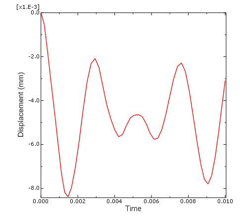
The truss responds dynamically to the load. You can confirm this by plotting the vertical displacement history of the node set CENTER.
You can create X–Y curves from either history or field data stored in the output database (.odb) file. X–Y curves can also be read from an external file or they can be typed into Abaqus/Viewer interactively. Once curves have been created, their data can be further manipulated and plotted to the screen in graphical form. In this example you will create and plot the curve using history data.
To create an X–Y plot of the vertical displacement for a node:
In the Results Tree, expand the History Output container underneath the output database named frame_xpl.odb.
From the list of available history output, double-click Spatial displacement: U2 at Node 102 in NSET CENTER.
Abaqus/Viewer plots the vertical displacement at the center node along the bottom of the truss, as shown in Figure 2–15.
Note:
The chart legend has been suppressed and the axis labels modified in this figure. Many X–Y plot options are directly accessible by double-clicking the appropriate regions of the viewport. To enable direct object actions, however, you must first click ![]() in the prompt area to cancel the current procedure (if necessary). To suppress the legend, double-click it in the viewport to open the Chart Legend Options dialog box. In the Contents tabbed page of this dialog box, toggle off Show legend. To modify the axis labels, double-click either axis to open the Axis Options dialog box, and edit the axis titles as indicated in Figure 2–15.
in the prompt area to cancel the current procedure (if necessary). To suppress the legend, double-click it in the viewport to open the Chart Legend Options dialog box. In the Contents tabbed page of this dialog box, toggle off Show legend. To modify the axis labels, double-click either axis to open the Axis Options dialog box, and edit the axis titles as indicated in Figure 2–15.
Exiting Abaqus/Viewer
Save your model database file; then select File![]() Exit from the main menu bar to exit Abaqus/Viewer.
Exit from the main menu bar to exit Abaqus/Viewer.