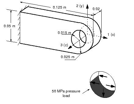
In this example you will use three-dimensional, continuum elements to model the connecting lug shown in Figure 4–14.
The lug is welded firmly to a massive structure at one end. The other end contains a hole. When it is in service, a bolt will be placed through the hole of the lug. You have been asked to determine the static deflection of the lug when a 30 kN load is applied to the bolt in the negative 2-direction. Because the goal of this analysis is to examine the static response of the lug, you should use Abaqus/Standard as your analysis product. You decide to simplify this problem by making the following assumptions:
Rather than include the complex bolt-lug interaction in the model, you will use a distributed pressure over the bottom half of the hole to load the connecting lug (see Figure 4–14).
You will neglect the variation of pressure magnitude around the circumference of the hole and use a uniform pressure.
The magnitude of the applied uniform pressure will be 50 MPa: 30 kN/ (2 × 0.015 m × 0.02 m).
After examining the static response of the lug, you will modify the model and use Abaqus/Explicit to study the transient dynamic effects resulting from sudden loading of the lug.
In your model define the global 1-axis to lie along the length of the lug, the global 2-axis to be vertical, and the global 3-axis to lie in the thickness direction. Place the origin of the global coordinate system (![]() ) at the center of the hole on the
) at the center of the hole on the ![]() face (see Figure 4–14).
face (see Figure 4–14).
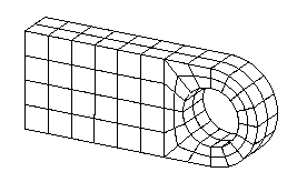
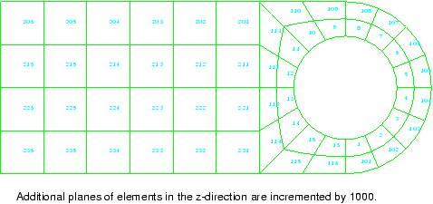
You need to consider the type of element that will be used before you start building the mesh for a particular problem. A suitable mesh design that uses quadratic elements may very well be unsuitable if you change to linear, reduced-integration elements. For this example use 20-node hexahedral elements with reduced integration (C3D20R). With the element type selected, you can design the mesh for the connecting lug. The most important decision regarding the mesh design for this application is how many elements to use around the circumference of the lug's hole. A possible mesh for the connecting lug is shown in Figure 4–15; you should build your model to be similar to it.
Another thing to consider when designing a mesh is what type of results you want from the simulation. The mesh in Figure 4–15 is rather coarse and, therefore, unlikely to yield accurate stresses. Four quadratic elements per 90° is the minimum number that should be considered for a problem like this one; using twice that many is recommended to obtain reasonably accurate stress results. However, this mesh should be adequate to predict the overall level of deformation in the lug under the applied loads, which is what you were asked to determine. The influence of increasing the mesh density used in this simulation is discussed in “Mesh convergence,” Section 4.4.
You need to decide what system of units to use in your model. The SI system of meters, seconds, and kilograms is recommended, but use another system if you prefer.
The model for the overhead hoist in Chapter 2, “Abaqus Basics,” was simple enough that the Abaqus input file could be created by typing the input directly into a text editor. This approach clearly is impractical for most real problems; instead, this example and all subsequent examples in the book point you to the completed input file for the example, and the steps in the examples illustrate the syntax of model and history data in the Abaqus input file. The complete input file for this example, lug.inp, is available in “Connecting lug,” Section A.2.
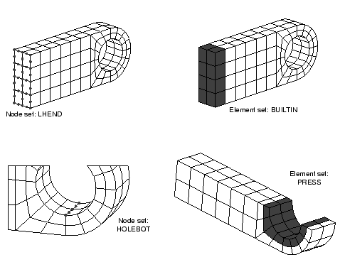
This example uses the mesh, the node and element sets shown in Figure 4–16, and the pressure load and boundary conditions shown in Figure 4–14.
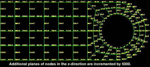
Subsequent steps will add the additional data needed for the model to describe the format of an Abaqus input file. If you would prefer to adjust the mesh and you do not have a preprocessor, use the Abaqus mesh generation options in “Connecting lug,” Section A.2. If you wish to create the entire model using Abaqus/CAE, refer to “Example: connecting lug,” Section 4.3 of Getting Started with Abaqus: Interactive Edition.In the description of this simulation that follows, the node and element numbers used are from the model found in “Connecting lug,” Section A.2. These node and element numbers are shown in Figure 4–17 and Figure 4–18. If you use a preprocessor, the node and element numbering in your model will almost certainly differ from that shown here. As you make modifications to your input file, remember to use the node and element numbers in your model and not those given here.
The model data—including the node and element definitions, set definitions, and section and material properties—are discussed in the following sections.
Model description
An Abaqus input file always starts with the *HEADING option. Often the description given in this option by the preprocessor is not very informative, although it might give the date and time when the file was generated. You should provide a suitable title on the data lines of this option so that someone looking at this file can tell what is being modeled and what units you used. The *HEADING option block used in lug.inp appears below:
*HEADING
Linear Elastic Steel Connecting Lug
S.I. Units (N, kg, m, s)
Nodal coordinates and element connectivity
In input files created by a preprocessor, the model's nodal coordinates usually are in one large *NODE option block, with the coordinates specified for each node individually.
The element definitions generated by the preprocessor usually are contained in several *ELEMENT option blocks. Typically, each block contains elements that have the same element section and material properties. In the connecting lug model only one element type is used, and all the elements have the same properties. Therefore, there will probably be a single *ELEMENT option block in your input file. It will look similar to
*ELEMENT, TYPE=C3D20R, ELSET=LUG
   1,     1,   401,   405,     5, 10001, 10401, 10405, 10005,
 201,   403,   205,     3, 10201, 10403, 10205, 10003,
5001,  5401,  5405,  5005
   2,     5,   405,   409,     9, 10005, 10405, 10409, 10009,
 205,   407,   209,     7, 10205, 10407, 10209, 10007,
5005,  5405,  5409,  5009
.......
Here three data lines are used to define the connectivity of one C3D20R element completely (a minimum of two is required). If a data line in an *ELEMENT option block ends with a comma, it indicates that the next data line contains more nodes defining the current element. The parameter ELSET=LUG indicates that all the elements defined in the following data lines will be stored in an element set called LUG. If your model does not have a descriptive element set name in the *ELEMENT option, change it to LUG.
Node and element sets
The node and element sets are important components of an Abaqus input file because they allow you to assign loads, boundary conditions, and material properties efficiently. They also offer great flexibility in defining the output that your simulation will produce and make it much easier to understand the input file.
Some preprocessors, such as Abaqus/CAE, will allow you to select and name groups of entities, such as nodes and elements, as you build the model; when the Abaqus input file is created, node and element sets are generated from these groups.
You define sets using the *NSET and *ELSET options in the input file. The name of a set is specified with either the NSET or ELSET parameter. The data lines list the nodes or elements that are included in the set. Each data line can contain up to 16 numbers, and there can be as many data lines as required. For example, the node set LHEND (see Figure 4–16) can be defined as
*NSET, NSET=LHEND
 3241,  3243,  3245,  3247,  3249,  3251,  3253,  3255, 3257,
 8241,  8245,  8249,  8253,  8257, 13241, 13243, 13245, 13247,
13249, 13251, 13253, 13255, 13257, 18241, 18245, 18249, 18253,
18257, 23241, 23243, 23245, 23247, 23249, 23251, 23253, 23255,
23257
If you are adding a node or element set to the input file with an editor and the identification numbers follow a regular pattern, the GENERATE parameter allows a range of nodes to be included by specifying the beginning node number, ending node number, and the increment in node numbers. For example, the node set LHEND could be defined as follows:
*NSET, NSET=LHEND, GENERATE
 3241,  3257, 2
 8241,  8257, 4
13241, 13257, 2
18241, 18257, 4
23241, 23257, 2
Sets can also be created by referring to other sets. If the preprocessor that you used did not create the element set BUILTIN or the node set HOLEBOT that are shown in Figure 4–16, add them to your input file using an editor; they will be essential in limiting the output during the simulation. You should also create the element set PRESS shown in Figure 4–16. Remember to use the node and element numbers in your model and not those shown in the figure.
Section properties
Look up the C3D20R element in Chapter 28, “Continuum Elements,” of the Abaqus Analysis User's Guide to determine the correct element section option and the required data that must be specified for this element. You will discover that the C3D20R element uses the *SOLID SECTION option to define the element's section properties. Because this is a three-dimensional element, Abaqus needs no additional geometric data for the element section.
Element set LUG contains all the elements, so that element set is suitable for this example. The following element section option statement is used for this example:
*SOLID SECTION, ELSET=LUG, MATERIAL=STEEL
If you did not define an element set with the name LUG, use the name of whatever element set contains all the elements in your model as the value of the ELSET parameter. The material property definition in the model will have the name STEEL.
Materials
The connecting lug is made of a mild steel and, thus, has isotropic, linear elastic material behavior under the loads being applied. Assume that E = 200 GPa and that ![]() = 0.3. These are given on the data line of the *ELASTIC option (remember the overhead hoist example in Chapter 2, “Abaqus Basics”). The following material property definition specifies these properties in the input file:
= 0.3. These are given on the data line of the *ELASTIC option (remember the overhead hoist example in Chapter 2, “Abaqus Basics”). The following material property definition specifies these properties in the input file:
*MATERIAL, NAME=STEEL
*ELASTIC
200.E9, 0.3
The value for the NAME parameter on the *MATERIAL option must match the value of the MATERIAL parameter on the *SOLID SECTION option.
The history data portion of the input file starts at the first *STEP option. Many preprocessors create a linear static step in the input file by default. This example will use a general static step. The following options define the step:
*STEP
<possibly a title describing this step>
*STATIC
If these options are not in your input file, add them at the end of the existing data. It is easier for someone else to understand your model if you use the data lines following the *STEP option to add a suitable title describing the event being simulated in the step.
Boundary conditions
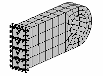
In the model of the connecting lug, all the nodes need to be constrained in all three directions at the left-hand end where it is attached to its parent structure (see Figure 4–19).
In this example, each constrained degree of freedom is specified individually in the *BOUNDARY option block, as shown below:
*BOUNDARY
3241, 1,1
3241, 2,2
3241, 3,3
......
If a large number of nodes are constrained, these data can occupy a great deal of space in the computer's memory. Where a number of nodes all have the same boundary conditions, it is more efficient to apply the constraints directly to a node set containing all the nodes. Thus, in the lug model we prefer to create the node set LHEND to specify the constraints:
*BOUNDARY
LHEND, ENCASTRE
If you think that you defined the boundary conditions incorrectly, you can display them in Abaqus/Viewer and compare them with the boundary conditions shown in Figure 4–19. The postprocessing instructions given at the end of “Postprocessing,” Section 2.3.9, discuss how to do this.
Loading
The lug carries a pressure of 50 MPa distributed around the bottom-half of the hole. Pressure loads can be defined conveniently using the preprocessor by selecting the element faces to which the load is applied. In the connecting lug input file, these loads will appear as a *DLOAD option block. For example, the *DLOAD option block for the connecting lug may look like
*DLOAD
   1,  P6, 5.E+07
   2,  P6, 5.E+07
   3,  P6, 5.E+07
   4,  P6, 5.E+07
  13,  P6, 5.E+07
...

1015,  P6, 5.E+07
1016,  P6, 5.E+07
The format of each data line is
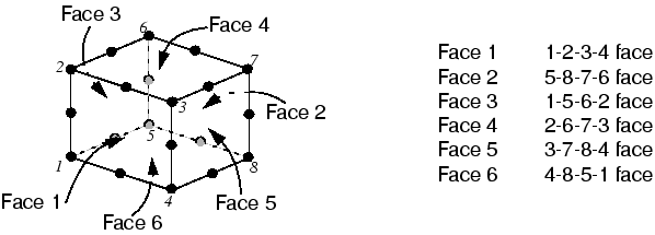
<element or element set name>, <load ID>, <load magnitude>In this case the “load ID” consists of the letter “P” followed by the number of the element face to which pressure is applied. The face numbers depend on the connectivity of the element and are defined for each element type in the Abaqus Analysis User's Guide. For the three-dimensional hexahedral elements used in this example, the face numbers are shown in Figure 4–20. In the model, as defined in “Connecting lug,” Section A.2, the pressure is applied to face 6 of the elements around the bottom of the hole, so the load ID is “P6.”
For meshes generated with a preprocessor, the face numbers and, hence, the load IDs will depend on how the mesh is generated. Some preprocessors, such as Abaqus/CAE, can determine the correct load ID automatically; this makes it very easy to specify pressure loads on complicated meshes. However, this method tends to produce long lists of data lines in the input file. In models where the same load ID and load magnitude are used for each element, you can use an element set—which is more efficient—to apply the pressure loads. For example, in this model the *DLOAD option block may appear as
*DLOAD
PRESS,  P6, 5.E+07
where we have made use of the element set PRESS whose members are shown in Figure 4–16.
Output requests
By default, many preprocessors create an Abaqus input file that has a large number of output request options. These requests are in addition to the output database file request that is generated automatically by Abaqus. If, when you edit your input file, you find that these additional output options were created, delete them because they will generally generate too much unnecessary output.
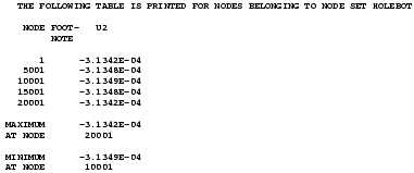
You were asked to determine the deflection of the connecting lug when the load is applied. A simple method for obtaining this result is to print out all the displacements in the model. However, it is likely that the location on the lug with the largest deflection is probably going to be on the bottom of the hole, where the load is applied. Furthermore, only the displacement in the 2-direction (U2) is going to be of interest. You should have created a node set, HOLEBOT, containing those nodes. Use that set to limit the requested displacements to just those five nodes at the bottom of the hole and to limit the output to just the vertical displacements.
*NODE PRINT, NSET=HOLEBOT
U2,
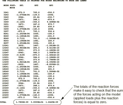
It is good practice to check that the reaction forces at the constraints balance the applied loads. All the reaction forces at a node can be printed by specifying the variable RF. We again use the node set LHEND to limit the output to those nodes that are constrained.
*NODE PRINT, NSET=LHEND, TOTAL=YES, SUMMARY=NO
RF,
You can define several *NODE PRINT and *EL PRINT options. The parameter TOTALS=YES causes the sum of the reaction forces at all the nodes in the node set to be printed. The SUMMARY=NO parameter prevents the minimum and maximum values in the table from being printed.
The following commands print the stress tensor (variable S) and the Mises stress (variable MISES) for the elements at the constrained end (element set BUILTIN):
*EL PRINT, ELSET=BUILTIN
S, MISES
You will use the NFORC output variable to create and display free body cuts in “Postprocessing—visualizing the results,” Section 4.3.8. The following options write the nodal forces due to the element stresses to the output database while also writing the default output:
*OUTPUT, FIELD, VARIABLE=PRESELECT
*ELEMENT OUTPUT
NFORC,
*OUTPUT, HISTORY, VARIABLE=PRESELECT
The end of a step is indicated with the option
*END STEPThis input option must be the last option in your model.
If you modified any input data, store the input in a file called lug.inp (an example file is listed in “Connecting lug,” Section A.2). Then, run the simulation using the command:
abaqus job=lug interactive
When the job has completed, check the data file, lug.dat, for any errors or warnings. If there are any errors, correct the input file and run the simulation again. If you have problems correcting any errors, try comparing your input file to the one given in “Connecting lug,” Section A.2. Check that you have the correct parameters for each input option.
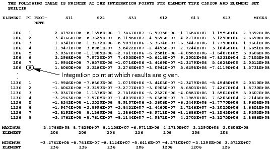
When the job has completed successfully, look at the three tables of output that you requested. They will be found at the end of the data file. A portion of the table of element stresses is shown in Figure 4–21. The maximum Mises stress at the built-in end is approximately 306 MPa.
The tables showing the displacements of the nodes along the bottom of the hole and the reaction forces at the constrained nodes are shown in Figure 4–22 and Figure 4–23, respectively.
The bottom of the hole in the lug has displaced about 0.3 mm. The total reaction force in the 2-direction at the constrained nodes is equal and opposite to the applied load in that direction of 30 kN.Once you have looked at the results in the data file, start Abaqus/Viewer by typing the following command at the operating system prompt:
abaqus viewer odb=lug
Plotting the deformed shape
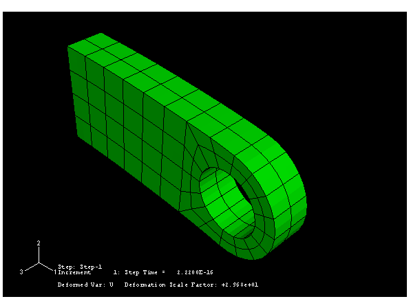
From the main menu bar, select Plot![]() Deformed Shape; or use the
Deformed Shape; or use the ![]() tool in the toolbox. Figure 4–24 displays the deformed model shape at the end of the analysis. What is the displacement magnification level?
tool in the toolbox. Figure 4–24 displays the deformed model shape at the end of the analysis. What is the displacement magnification level?
Changing the view
The default view is isometric. You can change the view using the options in the View menu or the view tools in the View Manipulation toolbar. You can also specify a view by entering values for rotation angles, viewpoint, zoom factor, or fraction of viewport to pan. Direct view manipulation is also available using the 3D compass.
To manipulate the view using the 3D compass:
Click and drag one of the straight axes of the 3D compass to pan along an axis.
Click and drag any of the quarter-circular faces on the 3D compass to pan along a plane.
Click and drag one of the three arcs along the perimeter of the 3D compass to rotate the model about the axis that is perpendicular to the plane containing the arc.
Click and drag the free rotation handle (the point at the top of the 3D compass) to rotate the model freely about its pivot point.
Click the label for any of the axes on the 3D compass to select a predefined view (the selected axis is perpendicular to the plane of the viewport).
Double-click anywhere on the 3D compass to specify a view.
To specify the view:
From the main menu bar, select View![]() Specify (or double-click the 3D compass).
Specify (or double-click the 3D compass).
The Specify View dialog box appears.
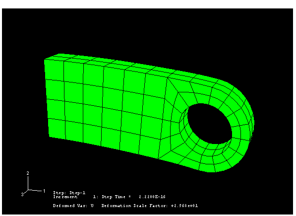
From the list of available methods, select Viewpoint.
In the Viewpoint method, you enter three values representing the X-, Y-, and Z-position of an observer. You can also specify an up vector. Abaqus positions your model so that this vector points upward.
Enter the X-, Y-, and Z-coordinates of the viewpoint vector as 1, 1, 3 and the coordinates of the up vector as 0, 1, 0.
Click OK.
Abaqus/Viewer displays your model in the specified view, as shown in Figure 4–25.
Visible edges
Several options are available for choosing which edges will be visible in the model display. The previous plots show all exterior edges of the model; Figure 4–26 displays only feature edges.
To display only feature edges:
From the main menu bar, select Options![]() Common.
Common.
The Common Plot Options dialog box appears.
Click the Basic tab if it is not already selected.
From the Visible Edges options, choose Feature edges.
Click Apply.
The deformed plot in the current viewport changes to display only feature edges, as shown in Figure 4–26.
Render style
A shaded plot is a filled plot in which a lightsource appears to be directed at the model. This is the default render style and can be very useful when viewing complex three-dimensional models. Three other render styles provide additional display options: wireframe, hidden line, and filled. You can select a render style from the Common Plot Options dialog box or from the tools on the Render Style toolbar: wireframe ![]() , hidden line
, hidden line ![]() , filled
, filled ![]() , and shaded
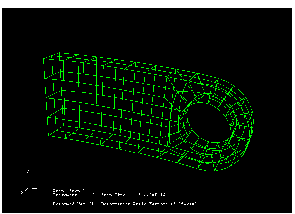
, and shaded ![]() . To display the wireframe plot shown in Figure 4–27, select Exterior edges in the Common Plot Options dialog box, click OK to close the dialog box, and select wireframe plotting by clicking the
. To display the wireframe plot shown in Figure 4–27, select Exterior edges in the Common Plot Options dialog box, click OK to close the dialog box, and select wireframe plotting by clicking the ![]() tool. All subsequent plots will be displayed in the wireframe render style until you select another render style.
tool. All subsequent plots will be displayed in the wireframe render style until you select another render style.
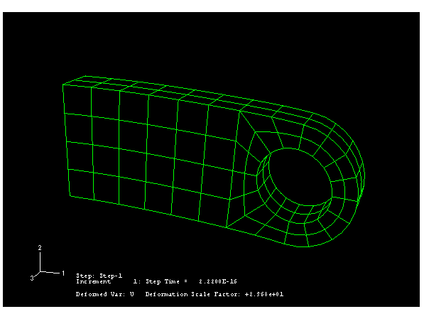
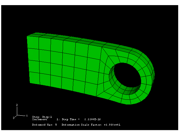
A wireframe model showing internal edges can be visually confusing for complex three-dimensional models. You can use the other render style tools to select the hidden line and filled render styles, shown in Figure 4–28 and Figure 4–29, respectively. These render styles are more useful when viewing complex three-dimensional models.
Contour plots
Contour plots display the variation of a variable across the surface of a model. You can create filled or shaded contour plots of field output results from the output database.
To generate a contour plot of the Mises stress:
From the main menu bar, select Plot![]() Contours
Contours![]() On Deformed Shape.
On Deformed Shape.
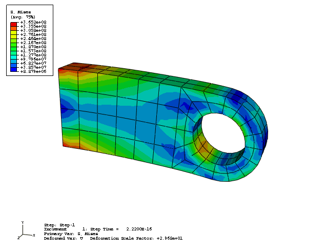
The filled contour plot shown in Figure 4–30 appears.
The Mises stress, S Mises, indicated in the legend title is the default variable chosen by Abaqus for this analysis. You can select a different variable to plot.
From the main menu bar, select Result![]() Field Output.
Field Output.
The Field Output dialog box appears; by default, the Primary Variable tab is selected.
From the list of available output variables, select a new variable to plot.
Click OK.
The contour plot in the current viewport changes to reflect your selection.
Tip: You can also use the Field Output toolbar, located above the viewport, to change the displayed field output variable. For more information, see “Using the field output toolbar,” Section 42.5.2 of the Abaqus/CAE User's Guide.
Abaqus/Viewer offers many options to customize contour plots. To see the available options, click the Contour Options ![]() tool in the toolbox. By default, Abaqus/Viewer automatically computes the minimum and maximum values shown in your contour plots and evenly divides the range between these values into 12 intervals. You can control the minimum and maximum values Abaqus/Viewer displays (for example, to examine variations within a fixed set of bounds), as well as the number of intervals.
tool in the toolbox. By default, Abaqus/Viewer automatically computes the minimum and maximum values shown in your contour plots and evenly divides the range between these values into 12 intervals. You can control the minimum and maximum values Abaqus/Viewer displays (for example, to examine variations within a fixed set of bounds), as well as the number of intervals.
To generate a customized contour plot:
In the Basic tabbed page of the Contour Plot Options dialog box, drag the Contour Intervals slider to change the number of intervals to nine.
In the Limits tabbed page of the Contour Plot Options dialog box, choose Specify beside Max; then enter a maximum value of 400E+6.
Choose Specify beside Min; then enter a minimum value of 60E+6.
Click OK.
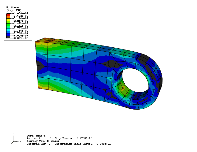
Abaqus/Viewer displays your model with the specified contour option settings, as shown in Figure 4–31 (this figure shows Mises stress; your plot will show whichever output variable you have chosen). These settings remain in effect for all subsequent contour plots until you change them or reset them to their default values.
Displaying contour results on interior surfaces
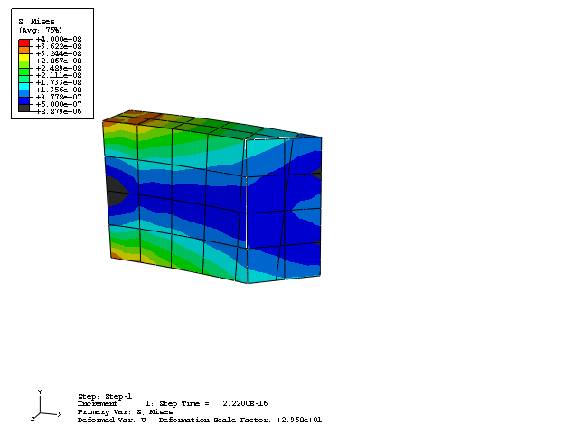
You can cut your model such that interior surfaces are made visible. For example, you may want to examine the stress distribution in the interior of a part. View cuts can be created for such purposes. Here, a simple planar cut is made through the lug to view the Mises stress distribution through the thickness of the part.
To create a view cut:
From the main menu bar, select Tools![]() View Cut
View Cut![]() Create.
Create.
In the dialog box that appears, accept the default name and shape. Enter 0,0,0 as the Origin of the plane (i.e., a point through which the plane will pass), 1,0,1 as the Normal axis to the plane, and 0,1,0 as Axis 2 of the plane.
Click OK to close the dialog box and to make the view cut.
The view appears as shown in Figure 4–32.
From the main menu bar, select ToolsTo view the full model again, toggle off Cut-4 in the View Cut Manager.
For more information on view cuts, see Chapter 80, “Cutting through a model,” of the Abaqus/CAE User's Guide.
Maximum and minimum values
The maximum and minimum values of a variable in a model can be determined easily.
To display the minimum and maximum values of a contour variable:
From the main menu bar, select Viewport![]() Viewport Annotation Options; then click the Legend tab in the dialog box that appears.
Viewport Annotation Options; then click the Legend tab in the dialog box that appears.
The Legend options become available.
Toggle on Show min/max values.
Click OK.
The contour legend changes to report the minimum and maximum contour values.
One of the goals of this example is to determine the deflection of the lug in the negative 2-direction. You can contour the displacement component of the lug in the 2-direction to determine its peak displacement in the vertical direction as follows. In the Contour Plot Options dialog box, click Defaults to reset the minimum and maximum contour values and the number of intervals to their default values before proceeding.
To contour the displacement of the connecting lug in the 2-direction:
From the list of variable types on the left side of the Field Output toolbar, select Primary if it is not already selected.
Tip:
You can click ![]() on the left side of the Field Output toolbar to make your selections from the Field Output dialog box instead of the toolbar. If you use the dialog box, you must click Apply or OK for Abaqus/Viewer to display your selections in the viewport.
on the left side of the Field Output toolbar to make your selections from the Field Output dialog box instead of the toolbar. If you use the dialog box, you must click Apply or OK for Abaqus/Viewer to display your selections in the viewport.
From the list of available output variables in the center of the toolbar, select output variable U.
From the list of available components and invariants on the right side of the Field Output toolbar, select U2.
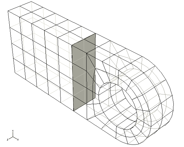
Displaying a subset of the model
By default, Abaqus/Viewer displays your entire model; however, you can choose to display a subset of your model called a display group. This subset can contain any combination of part instances, geometry (cells, faces, or edges), elements, nodes, and surfaces from the current model or output database. For the connecting lug model you will create a display group consisting of the elements at the bottom of the hole. Since a pressure load was applied to this region, an internal set is created by Abaqus that can be used for visualization purposes.
To display a subset of the model:
In the Results Tree, double-click Display Groups.
The Create Display Group dialog box opens.
From the Item list, select Elements. From the Method list, select Internal sets.
Once you have selected these items, the list on the right-hand side of the Create Display Group dialog box shows the available selections.
Using this list, identify the set that contains the elements at the bottom of the hole. Toggle on Highlight items in viewport below the list so that the outlines of the elements in the selected set are highlighted in red.
When the highlighted set corresponds to the group of elements at the bottom of the hole, click Replace ![]() to replace the current model display with this element set.
to replace the current model display with this element set.
Abaqus/Viewer displays the specified subset of your model.
Click Dismiss to close the Create Display Group dialog box.
When creating an Abaqus model, you may want to determine the face labels for a solid element. For example, you may want to verify that the correct load ID was used when applying pressure loads or when defining surfaces for contact. In such situations you can use the Visualization module to display the mesh after you have run a datacheck analysis that creates an output database file.
To display the face identification labels and element numbers on the undeformed model shape:
From the main menu bar, select Options![]() Common.
Common.
The Common Plot Options dialog box appears.
Set the render style to filled; all visible element edges will be displayed for convenience.
Toggle on Filled under Render Style.
Toggle on All edges under Visible Edges.
Click the Labels tab, and toggle on Show element labels and Show face labels.
Click Apply to apply the plot options.
From the main menu bar, select Plot![]() Undeformed Shape; or use the
Undeformed Shape; or use the ![]() tool in the toolbox.
tool in the toolbox.
Abaqus/Viewer displays the element and face identification labels in the current display group.
Click Defaults in the Common Plot Options dialog box to restore the default plot settings and then click OK to close the dialog box.
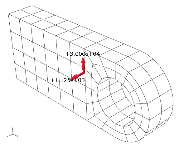
Displaying a free body cut
You can define a free body cut to view the resultant forces and moments transmitted across a selected surface of a model. Force vectors are displayed with a single arrowhead and moment vectors with a double arrowhead.
To create a free body cut:
To display the entire model in the viewport, select Tools![]() Display Group
Display Group![]() Plot
Plot![]() All from the main menu bar.
All from the main menu bar.
From the main menu bar, select Tools![]() Free Body Cut
Free Body Cut![]() Manager.
Manager.
Click Create in the Free Body Cut Manager.
From the dialog box that appears, select 3D element faces as the Selection method and click Continue.
In the Free Body Cross-Section dialog box, select Surfaces as the Item and Pick from viewport as the Method.
In the prompt area, set the selection method to by angle and accept the default angle.
Select the surface, highlighted in Figure 4–33, to define the free body cut cross-section.
From the Selection toolbar, toggle off the Select the Entity Closest to the Screen tool ![]() and ensure that the Select From All Entities tool
and ensure that the Select From All Entities tool ![]() is selected.
is selected.
As you move the cursor in the viewport, Abaqus/CAE highlights all of the potential selections and adds ellipsis marks (...) next to the cursor arrow to indicate an ambiguous selection. Position the cursor so that one of the faces of the desired surface is highlighted, and click to display the first surface selection.
Use the Next and Previous buttons to cycle through the possible selections until the appropriate vertical surface is highlighted, and click OK.
Click Done in the prompt area to indicate your selection is complete. Click OK in the Free Body Cross-Section dialog box.
In the Edit Free Body Cut dialog box, accept the default settings for the Summation Point and the Component Resolution. Click OK to close the dialog box.
Click Options in the Free Body Cut Manager.
From the Free Body Plot Options dialog box, select the Force tab in the Color & Style tabbed page. Click the resultant color sample ![]() to change the color of the resultant force arrow.
to change the color of the resultant force arrow.
Once you have selected a new color for the resultant force arrow, click OK in the Free Body Plot Options dialog box and click Dismiss in the Free Body Cut Manager.
The free body cut is displayed in the viewport, as shown in Figure 4–34.
Generating tabular data reports for subsets of the model
Tabular output data were generated earlier for this model using printed output requests. However, for complicated models it is convenient to write these data for selected regions of the model using Abaqus/Viewer. This is achieved using display groups in conjunction with the report generation feature. For the connecting lug problem we will generate the following tabular data reports:
Stresses in the elements at the built-in end of the lug (to determine the maximum stress in the lug)
Reaction forces at the built-in end of the lug (to check that the reaction forces at the constraints balance the applied loads)
Vertical displacements at the bottom of the hole (to determine the deflection of the lug when the load is applied)
Each of these reports will be generated using display groups whose contents are selected in the viewport. Thus, begin by creating and saving display groups for each region of interest.
To create and save a display group containing the elements at the built-in end:
In the Results Tree, double-click Display Groups.
Choose Elements from the Item list and Pick from viewport as the selection method.
Restore the option to select entities closest to the screen.
In the prompt area, set the selection method to by angle; and click the built-in face of the lug. Click Done when all the elements at the built-in face of the lug are highlighted in the viewport. In the Create Display Group dialog box, click Save Selection As. Save the display group as built-in elements.
To create and save a display group containing the nodes at the built-in end:
In the Create Display Group dialog box, choose Nodes from the Item list and Pick from viewport as the selection method.
In the prompt area, set the selection method to by angle; and click the built-in face of the lug. Click Done when all the nodes on the built-in face of the lug are highlighted in the viewport. In the Create Display Group dialog box, click Save Selection As. Save the display group as built-in nodes.
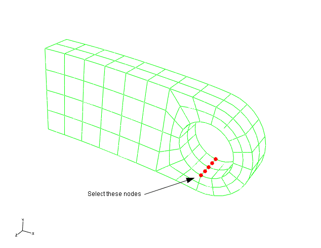
To create and save a display group containing the nodes at the bottom of the hole:
In the Create Display Group dialog box, click Edit Selection to select a different group of nodes.
In the prompt area, set the selection method to individually; and select the nodes at the bottom of the hole in the lug, as indicated in Figure 4–35. Click Done when all the nodes on the bottom of the hole are highlighted in the viewport. In the Create Display Group dialog box, click Save Selection As. Save the display group as nodes at hole bottom.
Now generate the reports.
To generate field data reports:
In the Results Tree, click mouse button 3 on built-in elements underneath the Display Groups container. In the menu that appears, select Plot to make it the current display group.
From the main menu bar, select Report![]() Field Output.
Field Output.
In the Variable tabbed page of the Report Field Output dialog box, accept the default position labeled Integration Point. Click the triangle next to S: Stress components to expand the list of available variables. From this list, select Mises and the six individual stress components: S11, S22, S33, S12, S13, and S23.
In the Setup tabbed page, name the report Lug.rpt. In the Data region at the bottom of the page, toggle off Column totals.
Click Apply.
In the Results Tree, click mouse button 3 on built-in nodes underneath the Display Groups container. In the menu that appears, select Plot to make it the current display group. (To see the nodes, toggle on Show node symbols in the Common Plot Options dialog box.)
In the Variable tabbed page of the Report Field Output dialog box, change the position to Unique Nodal. Toggle off S: Stress components, and select RF1, RF2, and RF3 from the list of available RF: Reaction force variables.
In the Data region at the bottom of the Setup tabbed page, toggle on Column totals.
Click Apply.
In the Results Tree, click mouse button 3 on nodes at hole bottom underneath the Display Groups container. In the menu that appears, select Plot to make it the current display group.
In the Variable tabbed page of the Report Field Output dialog box, toggle off RF: Reaction force, and select U2 from the list of available U: Spatial displacement variables.
In the Data region at the bottom of the Setup tabbed page, toggle off Column totals.
Click OK.
Open the file Lug.rpt in a text editor. A portion of the table of element stresses is shown below. The element data are given at the element integration points. The integration point associated with a given element is noted under the column labeled Int Pt. The bottom of the table contains information on the maximum and minimum stress values in this group of elements. The results indicate that the maximum Mises stress at the built-in end is approximately 330 MPa. Your results may differ slightly if your mesh is not identical to the one used here.
Field Output Report

Source 1
---------

   ODB: lug.odb
   Step: Step-1
   Frame: Increment      1: Step Time =   2.2200E-16

Loc 1 : Integration point values from source 1

Output sorted by column "Element Label".

Field Output reported at nodes for part: PART-1-1

Element   Int      S.Mises        S.S11        S.S22        S.S33        S.S12
Label     Pt        @Loc 1       @Loc 1       @Loc 1       @Loc 1       @Loc 1
------------------------------------------------------------------------------
        S.S13        S.S23
       @Loc 1       @Loc 1
--------------------------
  206     1    293.921E+06  281.921E+06  -8.1398E+06 -13.8667E+06 -6.99752E+06
 -11.6881E+06  1.15564E+06
  206     2      286.9E+06  347.661E+06  87.6292E+06  81.1577E+06 -49.8957E+06
  42.7097E+06  3.12903E+06
  206     3    196.605E+06  183.407E+06  1.32717E+06 -8.90914E+06  -33.674E+06
 -6.34469E+06  1.77895E+06
  206     4    168.508E+06  194.713E+06  38.9812E+06  38.4224E+06 -24.4931E+06
  27.2442E+06  3.10456E+06
  206     5    306.077E+06  303.672E+06 -1.19087E+06 -2.78165E+06  -8.2581E+06
 -4.05888E+06  -184.07E+03
  206     6    271.531E+06   329.68E+06  79.7248E+06  74.0551E+06 -56.4163E+06
  9.20019E+06 -78.3313E+03
  206     7    205.123E+06  199.438E+06  7.85751E+06 -1.07157E+06 -34.4693E+06
 -2.34785E+06  546.279E+03
  206     8    157.315E+06  180.601E+06  33.2797E+06  32.7648E+06 -30.9435E+06
  5.64979E+06 -74.1186E+03
    .
    .
  1236    1    205.096E+06 -199.458E+06 -7.88628E+06  1.07185E+06 -34.4032E+06
  -2.3479E+06 -545.449E+03
  1236    2    157.301E+06 -180.618E+06 -33.2934E+06 -32.7715E+06 -30.9083E+06
  5.65027E+06  74.2669E+03
  1236    3    306.071E+06  -303.67E+06  1.18777E+06  2.78175E+06  -8.2327E+06
 -4.05827E+06  185.017E+03
  1236    4     271.48E+06 -329.625E+06 -79.7048E+06 -74.0391E+06 -56.3889E+06
  9.19885E+06  78.2027E+03
  1236    5    196.584E+06 -183.433E+06 -1.35291E+06  8.91071E+06 -33.6059E+06
 -6.34491E+06 -1.77698E+06
  1236    6    168.507E+06 -194.738E+06  -38.996E+06 -38.4311E+06 -24.4598E+06
  27.2461E+06 -3.10252E+06
  1236    7    293.927E+06 -281.931E+06  8.13693E+06  13.8641E+06 -6.97109E+06
 -11.6862E+06 -1.15429E+06
  1236    8    286.857E+06 -347.614E+06 -87.6102E+06 -81.1438E+06 -49.8721E+06
  42.7034E+06 -3.12746E+06


  Minimum      35.7223E+06 -347.614E+06 -87.6102E+06 -81.1438E+06 -56.4163E+06
 -42.7097E+06 -3.12903E+06
      At Element       226          236          236         1236         1206
         1206         1206
          Int Pt         2            4            4            8            2
            6            6
  Maximum      306.077E+06  347.661E+06  87.6292E+06  81.1577E+06 -6.97109E+06
  42.7097E+06  3.12903E+06
      At Element       206         1206         1206          206         1236
          206          206
          Int Pt         5            6            6            2            7
            2            2
How does the maximum value of Mises stress compare to the value reported in the contour plot generated earlier? Do the two maximum values correspond to the same point in the model? The Mises stresses shown in the contour plot have been extrapolated to the nodes, whereas the stresses written to the report file for this problem correspond to the element integration points. Therefore, the location of the maximum Mises stress in the report file is not exactly the same as the location of the maximum Mises stress in the contour plot. This difference can be resolved by requesting that stress output at the nodes (extrapolated from the element integration points and averaged over all elements containing a given node) be written to the report file. If the difference is large enough to be of concern, this is an indication that the mesh may be too coarse.
The table listing the reaction forces at the constrained nodes is shown below. The Total entry at the bottom of the table contains the net reaction force components for this group of nodes. The results confirm that the total reaction force in the 2-direction at the constrained nodes is equal and opposite to the applied load of 30 kN in that direction.
Field Output Report

Source 1
---------

   ODB: lug.odb
   Step: Step-1
   Frame: Increment      1: Step Time =   2.2200E-16

Loc 1 : Nodal values from source 1

Output sorted by column "Node Label".

Field Output reported at nodes for part: PART-1-1

            Node          RF.RF1          RF.RF2          RF.RF3
           Label          @Loc 1          @Loc 1          @Loc 1
-----------------------------------------------------------------
            3241         872.912          765.17        -936.541
            3243    -10.7924E+03        -139.598    -2.69241E+03
            3245      2.5436E+03         29.2367        -636.668
            3247    -3.47143E+03         248.065        -879.401
            3249    -124.431E-03         -366.58     94.6864E-03
     .
     .
           23249    -124.431E-03         -366.58    -94.6864E-03
           23251     3.47251E+03         247.215        -879.699
           23253    -2.54332E+03         29.3956        -636.906
           23255     10.7918E+03        -139.991    -2.69226E+03
           23257        -873.161         765.137        -936.363


  Minimum           -18.4323E+03        -470.038    -2.69241E+03
         At Node           13243           13249            3243

  Maximum             18.431E+03      3.3654E+03     2.69241E+03
         At Node           13255            8241           23243

           Total     600.502E-06     30.0000E+03    -454.747E-12
The table showing the displacements of the nodes along the bottom of the hole (listed below) indicates that the bottom of the hole in the lug has displaced about 0.3 mm.
Field Output Report

Source 1
---------

   ODB: lug.odb
   Step: Step-1
   Frame: Increment      1: Step Time =   2.2200E-16

Loc 1 : Nodal values from source 1

Output sorted by column "Node Label".

Field Output reported at nodes for part: PART-1-1

            Node            U.U2
           Label          @Loc 1
---------------------------------
               1    -313.425E-06
           10001    -313.494E-06
           20001    -313.425E-06


  Minimum           -313.494E-06

         At Node           10001
  Maximum           -313.425E-06

At Node 20001You will now evaluate the dynamic response of the lug when the same load is applied suddenly. Of special interest is the transient response of the lug. You will have to modify the model for the Abaqus/Explicit analysis. Before proceeding, copy the existing input file to a input file named lug_xpl.inp. Make all subsequent changes to the lug_xpl.inp input file. Before running the explicit analysis, you will need to change the element type, add a density to the material model, and change the step type. In addition, you should make modifications to the field output requests.
Change element type
Second-order hexahedral elements are not available in the Abaqus/Explicit element library. Thus, you will need to change the element type specified on the *ELEMENT option from C3D20R to C3D8R. This change also requires that you edit the element nodal connectivity so that only eight nodes are specified for each element. For example, the following *ELEMENT option block was used to define one of the elements in lug.inp:
*ELEMENT, TYPE=C3D20R
   1,     1,   401,   405,     5, 10001, 10401, 10405, 10005,
 201,   403,   205,     3, 10201, 10403, 10205, 10003,
5001,  5401,  5405,  5005
In lug_xpl.inp this option block has two changes: the element type has been changed to C3D8R and the nodal connectivity consists of the first eight nodes in the original list, which define the corner nodes of the element.
*ELEMENT, TYPE=C3D8R
   1,     1,   401,   405,     5, 10001, 10401, 10405, 10005
Because the C3D8R element employs reduced integration, use the enhanced strain algorithm to control hourglassing. You can specify enhanced hourglassing with the *SECTION CONTROLS option:
*SOLID SECTION, ELSET=LUG, MATERIAL=STEEL, CONTROLS=EC-1
*SECTION CONTROLS, NAME=EC-1, HOURGLASS=ENHANCED
Edit the material definition
Since Abaqus/Explicit performs a dynamic analysis, a complete material definition requires that you specify the material density. For this problem assume the density is equal to 7800 kg/m3.
You can modify the material definition by adding the *DENSITY option to the material option block. The complete material definition for the connecting lug is:
*MATERIAL, NAME=STEEL
*ELASTIC
200.E9, 0.3
*DENSITY
7800.,
Replace the static step with a dynamic, explicit step
Revise the step definition to examine the dynamic response of the lug over a period of 0.005 s. This change requires that you change the *STEP option block, which appeared as follows for the static analysis:
*STEP
Apply uniform pressure to the hole
*STATIC
Replace this option block with the following one:
*STEP
Dynamic lug loading
*DYNAMIC, EXPLICIT
, 0.005
Request field output at evenly spaced intervals and default history output
Write field output at 125 equally spaced intervals and also write the default history output. You can specify output at evenly spaced intervals by appending the NUMBER INTERVAL parameter to the *OUTPUT option block. Replace the existing output requests with the following:
*OUTPUT, FIELD, NUMBER INTERVAL=125
*NODE OUTPUT
RF, U
*ELEMENT OUTPUT, DIRECTIONS=YES
S,
*OUTPUT, HISTORY, VARIABLE=PRESELECT
Save the changes to the input file called lug_xpl.inp. Then run the simulation using the command:
abaqus job=lug_xpl
In the static analysis performed with Abaqus/Standard you examined the deformed shape of the lug as well as stress and displacement output. For the Abaqus/Explicit analysis you can similarly examine the deformed shape, stresses, and displacements in the lug. Because transient dynamic effects may result from a sudden loading, you should also examine the time histories for internal and kinetic energy, displacement, and Mises stress.
Open the output database (.odb) file created by this job.
Plotting the deformed shape
From the main menu bar, select Plot![]() Deformed Shape; or use the
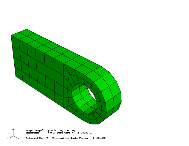
Deformed Shape; or use the ![]() tool in the toolbox. Figure 4–36 displays the deformed model shape at the end of the analysis.
tool in the toolbox. Figure 4–36 displays the deformed model shape at the end of the analysis.
To see the vibrations in the lug more clearly, change the deformation scale factor to 50. In addition, animate the time history of the deformed shape of the lug and decrease the frame rate of the time history animation.
The time history animation of the deformed shape of the lug shows that the suddenly applied load induces vibrations in the lug. Additional insights about the behavior of the lug under this type of loading can be gained by plotting the kinetic energy, internal energy, displacement, and stress in the lug as a function of time. Some of the questions to consider are:
Is energy conserved?
Was large-displacement theory necessary for this analysis?
Are the peak stresses reasonable? Will the material yield?
X–Y plotting
X–Y plots can display the variation of a variable as a function of time. You can create X–Y plots from field and history output.
To create X–Y plots of the internal and kinetic energy as a function of time:
In the Results Tree, expand the History Output container underneath the output database named lug_xpl.odb.
The list of all the variables in the history portion of the output database appears; these are the only history output variables you can plot.
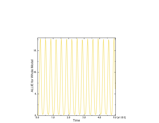
From the list of available output variables, double-click ALLIE to plot the internal energy for the whole model.
Abaqus reads the data for the curve from the output database file and plots the graph shown in Figure 4–37.
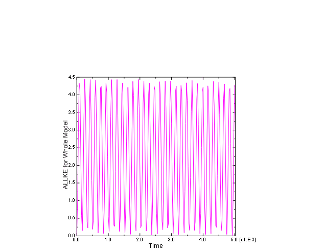
Repeat this procedure to plot ALLKE, the kinetic energy for the whole model (shown in Figure 4–38).
Both the internal energy and the kinetic energy show oscillations that reflect the vibrations of the lug. Throughout the simulation, kinetic energy is transformed into internal (strain) energy and vice-versa. Since the material is linear elastic, total energy is conserved. This can be seen by plotting ETOTAL, the total energy of the system, together with ALLIE and ALLKE. The value of ETOTAL is approximately zero throughout the course of the analysis. Energy balances in dynamic analysis are discussed further in Chapter 9, “Nonlinear Explicit Dynamics.”
To generate a plot of displacement versus time:
Plot the deformed shape of the lug. In the Results Tree, double-click XY Data.
In the Create XY Data dialog box that appears, select ODB field output as the source and click Continue.
In the XY Data from ODB Field Output dialog box that appears, select Unique Nodal as the type of position from which the X–Y data should be read.
Click the arrow next to U: Spatial displacement and toggle on U2 as the displacement variable for the X–Y data.
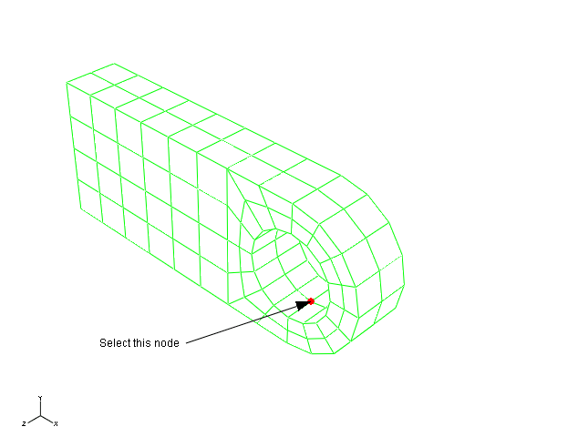
Select the Elements/Nodes tab. Choose Pick from viewport as the selection method for identifying the node for which you want X–Y data.
Click Edit Selection. In the viewport, select one of the nodes on the bottom of the hole as shown in Figure 4–39 (if necessary, change the render style to facilitate your selection). Click Done in the prompt area.
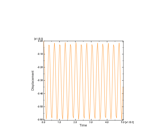
Click Plot in the XY Data from ODB Field Output dialog box to plot the nodal displacement as a function of time.
The history of the oscillation, as shown in Figure 4–40, indicates that the displacements are small (relative to the structure's dimensions).
Thus, this problem could have been solved adequately using small-deformation theory. This would have reduced the computational cost of the simulation without significantly affecting the results. Nonlinear geometric effects are discussed further in Chapter 8, “Nonlinearity.”
To generate a plot of Mises stress versus time:
Plot the deformed shape of the lug again.
Select the Variables tab in the XY Data from ODB Field Output dialog box. Deselect U2 as the variable for the X–Y data plot.
Change the Position field to Integration Point.
Click the arrow next to S: Stress components and toggle on Mises as the stress variable for the X–Y data.
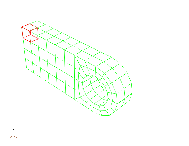
Select the Elements/Nodes tab. Choose Pick from viewport as the selection method for identifying the element for which you want X–Y data.
Click Edit Selection. In the viewport, select one of the elements near the built-in end of the lug as shown in Figure 4–41. Click Done in the prompt area.
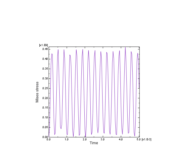
Click Plot in the XY Data from ODB Field Output dialog box to plot the Mises stress at the selected element as a function of time.
The peak Mises stress is on the order of 550 MPa, as shown in Figure 4–42. This value is larger than the typical yield strength of steel. Thus, the material would have yielded before experiencing such a large stress. Material nonlinearity is discussed further in Chapter 10, “Materials.”