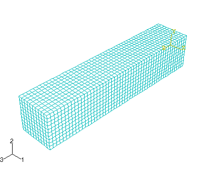
This example demonstrates some of the fundamental ideas in explicit dynamics described earlier in Chapter 2, “Abaqus Basics.” It also illustrates stability limits and the effect of mesh refinement and material properties on the solution time.
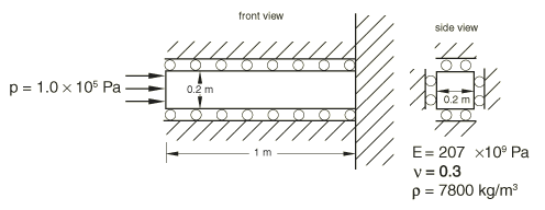
The bar has the dimensions shown in Figure 9–1.
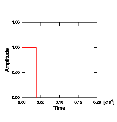
To make the problem a one-dimensional strain problem, all four lateral faces are on rollers; thus, the three-dimensional model simulates a one-dimensional problem. The material is steel with the properties shown in Figure 9–1. The free end of the bar is subjected to a blast load with a magnitude of 1.0 × 10⁵ Pa and a duration of 3.88 × 10⁵ s. The normalized load versus time is shown in Figure 9–2.Using the material properties (neglecting Poisson's ratio), we can calculate the wave speed of the material using the equations introduced in the previous section.
![]()
Create this mesh in your preprocessor. Use the coordinate system shown in Figure 9–3.
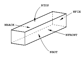
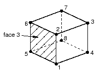
This example defines node and element sets to apply the loads and boundary conditions and to visualize output. The node sets are defined on their respective faces, as shown in Figure 9–4.
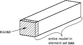
The element sets are defined as shown in Figure 9–5.
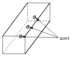
In addition, this example defined an element set containing three elements in the center of the bar. You can define this element set manually by selecting these elements such that their faces nearest to the free end are at distances 0.25 m, 0.5 m, and 0.75 m from the free end, as shown in Figure 9–6. These elements will be used for postprocessing.
In this section you will review your input file and include additional information.
Model description
The following would be a suitable description in the *HEADING option for this simulation:
*HEADING
Stress wave propagation in a bar -- 50x10x10 elements
SI units (kg, m, s, N)
Element connectivity
If you create input files using a preprocessor, check to make sure that you are using the correct element type (C3D8R). It is possible that the preprocessor specified the element type incorrectly. The *ELEMENT option block in this model begins with the following:
*ELEMENT, TYPE=C3D8R, ELSET=BAR
If you created this input file using a preprocessor, the name given for the ELSET parameter in your model may not be BAR. If necessary, change the name to BAR.
Section properties
The section properties are the same for all elements. In the following option statement, the element set BAR is used to assign the material properties to the elements.
*SOLID SECTION, ELSET=BAR, MATERIAL=STEEL
Material properties
The bar is made of steel, which we assume to be linear elastic with a Young's modulus of 207 × 109 Pa, a Poisson's ratio of 0.3, and a density of 7800 kg/m3. The following material option block specifies these values:
*MATERIAL, NAME=STEEL
*ELASTIC
207.0E9, 0.3
*DENSITY
7800.0,
Fixed boundary conditions
In this model, we fix all the translations at the built-in, right-hand end of the bar, then constrain the front, back, top, and bottom faces of the bar so that these faces are on rollers and the strain is uniaxial. Using the node sets defined previously, the following boundary conditions are used in this model:
*BOUNDARY
NFIX, 1, 3
NFRONT, 1, 1
NBACK, 1, 1
NTOP, 2, 2
NBOT, 2, 2
Amplitude definition
The blast load is applied at its maximum value instantaneously and is held constant for 3.88 × 10⁵ s. Then the load is suddenly removed and held constant at zero. The *AMPLITUDE option is used to define the time variation of loads and boundary conditions. On the data lines following the *AMPLITUDE option, pairs of data are given in the form:
<time>, <amplitude>, <time>, <amplitude>, etc.Up to four data pairs can be entered on each data line. Abaqus considers the amplitude to be held constant following the last amplitude value given. The following *AMPLITUDE option block defines the amplitude for the blast load:
*AMPLITUDE, NAME=BLAST
0., 1., 3.88E-5, 1., 3.89E-5, 0, 3.90E-5, 0.
We will now review the history data associated with this problem, including the step definition, loading, bulk viscosity, and output requests.
Step definition
The step definition indicates that this is an explicit dynamics analysis with a duration of 2.0 × 10⁴ s. You can also include a descriptive title for the step.
*STEP
Blast loading
*DYNAMIC, EXPLICIT
, 2.0E-4
Loading
Apply the pressure load with a value of 1.0 × 10⁵ Pa to the free face of the bar, which you previously defined to be in an element set called ELOAD. The pressure load at any given time is the magnitude specified under the *DLOAD option times the value interpolated from the amplitude curve. To apply the load correctly, you need to determine the face identifier label of the free element faces. For the model defined in “Stress wave propagation in a bar,” Section A.7, the free face is face number 3, which corresponds to the pressure identifier P3. The face identifier depends on the order in which the nodes are defined on the *ELEMENT option, as shown in Figure 9–7. Use the amplitude named BLAST when applying the pressure load.
*DLOAD, AMPLITUDE=BLAST
ELOAD, <P1, P2, P3, P4, P5, or P6>, 1.0E5
If you define the pressure load in your preprocessor, the correct face identifier should be determined automatically.
Bulk viscosity
To keep the stress wave as sharp as possible, the quadratic bulk viscosity (discussed in “Bulk viscosity,” Section 9.5.1) is set to zero.
*BULK VISCOSITY
0.06, 0.0
Output requests
By default, many preprocessors create an Abaqus input file that has a large number of output request options. If you created your input file using a preprocessor and you find that these default output options were created, delete them all because they will generally generate too much output.
You want to have an output database file created during the analysis so that you can use Abaqus/Viewer to postprocess the results. Four output database frames (intervals at which data are written to the output database) are adequate to show the stress wave propagating through the mesh. This example sets the parameter VARIABLE=PRESELECT on the *OUTPUT, FIELD option to write the default field data for a *DYNAMIC, EXPLICIT procedure to the output database file. In addition, stress (S) history output in element set EOUT is requested for every increment.
*OUTPUT, FIELD, VARIABLE=PRESELECT, NUMBER INTERVAL=4
*OUTPUT, HISTORY, FREQUENCY=1
*ELEMENT OUTPUT, ELSET=EOUT
S,
*END STEP
After storing your input in a file called wave_50x10x10.inp, run the analysis using the following command:
abaqus job=wave_50x10x10If your analysis does not complete, check the data file, wave_50x10x10.dat, and status file, wave_50x10x10.sta, for error messages. Modify your input file to remove the errors. If you still have trouble running your analysis, compare your input file to the one given in “Stress wave propagation in a bar,” Section A.7.
Status file
The status file, wave_50x10x10.sta, contains information about moments of inertia, followed by information concerning the initial stability limit. The 10 elements with the lowest stable time limits are listed in rank order.
   Most critical elements:
    Element number   Rank    Time increment   Increment ratio
   ----------------------------------------------------------
           1          1        2.237266E-06      1.000000E+00
          19          2        2.237266E-06      1.000000E+00
         201          3        2.237266E-06      1.000000E+00
         219          4        2.237266E-06      1.000000E+00
         301          5        2.237266E-06      1.000000E+00
         319          6        2.237266E-06      1.000000E+00
         501          7        2.237266E-06      1.000000E+00
         519          8        2.237266E-06      1.000000E+00
         601          9        2.237266E-06      1.000000E+00
         619         10        2.237266E-06      1.000000E+00
The status file continues with information about the progress of the solution.
 STEP 1  ORIGIN 0.0000

  Total memory used for step 1 is approximately 7.1 megabytes.
  Global time estimation algorithm will be used.
  Scaling factor:  1.0000
  Variable mass scaling factor at zero increment:  1.0000

              STEP     TOTAL       CPU      STABLE    CRITICAL    KINETIC      TOTAL
INCREMENT     TIME      TIME      TIME   INCREMENT     ELEMENT     ENERGY     ENERGY
        0  0.000E+00 0.000E+00  00:00:00 1.819E-06           1  0.000E+00  0.000E+00
Results number 0 at increment zero.
ODB Field Frame Number      0 of      4 requested intervals at increment zero.
ODB Field Frame Number      0 of      2 requested intervals at increment zero.
        5  1.119E-05 1.119E-05  00:00:00 2.237E-06         619  4.504E-05 -1.963E-06
       10  2.237E-05 2.237E-05  00:00:00 2.237E-06       20015  9.189E-05 -2.218E-06
       15  3.401E-05 3.401E-05  00:00:00 2.907E-06       20311  1.406E-04 -2.252E-06
       19  4.560E-05 4.560E-05  00:00:00 2.888E-06       20311  1.577E-04  1.009E-06
       21  5.137E-05 5.137E-05  00:00:00 2.882E-06       20911  1.556E-04  2.239E-06
ODB Field Frame Number      1 of      4 requested intervals at  5.137395E-05
       25  6.289E-05 6.289E-05  00:00:00 2.873E-06       20803  1.539E-04  1.713E-07.
.
.Start Abaqus/Viewer by typing the following command at the operating system prompt:
abaqus viewer odb=wave_50x10x10
Plotting the stress along a path
We are interested in looking at how the stress distribution along the length of the bar changes with time. To do so, we will look at the stress distribution at three different times throughout the course of the analysis.
Create a curve of the variation of the stress in the 3-direction (S33) along the axis of the bar for each of the first three frames of the output database file. To create these plots, you first need to define a straight path along the axis of the bar.
To create a point list path along the center of the bar:
In the Results Tree, double-click Paths.
The Create Path dialog box appears.
Name the path Center. Select Point list as the path type, and click Continue.
The Edit Point List Path dialog box appears.
In the Point Coordinates table, enter the coordinates of the centers of both ends of the bar. The input specifies a path from the first point to the second point, as defined in the global coordinate system of the model.
Note:
If you generated the geometry and mesh using the procedure described earlier, the table entries are 0, 0, 1 and 0, 0, 0. If you used an alternate procedure to generate the bar geometry, you can use the ![]() tool in the Query toolbar to determine the coordinates of the centers at each end of the bar.
tool in the Query toolbar to determine the coordinates of the centers at each end of the bar.
When you have finished, click OK to close the Edit Point List Path dialog box.
To save X–Y plots of stress along the path at three different times:
In the Results Tree, double-click XYData.
The Create XY Data dialog box appears.
Choose Path as the X–Y data source, and click Continue.
The XY Data from Path dialog box appears with the path that you created visible in the list of available paths. If the undeformed model shape is currently displayed, the path you select is highlighted in the plot.
Toggle on Include intersections under Point Locations.
Accept True distance as the selection in the X Values region of the dialog box.
Click Field Output in the Y Values region of the dialog box to open the Field Output dialog box.
Select the S33 stress component, and click OK.
The field output variable in the XY Data from Path dialog box changes to indicate that stress data in the 3-direction (S33) will be created.
Note: Abaqus/Viewer may warn you that the field output variable will not affect the current image. Leave the plot state As is, and click OK to continue.
Click Step/Frame in the Y Values region of the XY Data from Path dialog box.
In the Step/Frame dialog box that appears, choose frame 1, which is the second of the five recorded frames. (The first frame listed, frame 0, is the base state of the model at the beginning of the step.) Click OK.
The Y Values region of the XY Data from Path dialog box changes to indicate that data from Step 1, frame 1 will be created.
To save the X–Y data, click Save As.
The Save XY Data As dialog box appears.
Name the X–Y data S33_T1, and click OK.
S33_T1 appears in the XYData container of the Results Tree.
Repeat Steps 7 through 9 to create X–Y data for frames 2 and 3. Name the data sets S33_T2 and S33_T3, respectively.
To close the XY Data from Path dialog box, click Cancel.
To plot the stress curves:
In the XYData container, drag the cursor to select all three X–Y data sets.
Click mouse button 3, and select Plot from the menu that appears.
Abaqus/Viewer plots the stress in the 3-direction along the center of the bar for frames 1, 2, and 3, corresponding to approximate simulation times of 5 × 10⁵ s, 1 × 10⁴ s, and 1.5 × 10⁴ s, respectively.
Click ![]() in the prompt area to cancel the current procedure.
in the prompt area to cancel the current procedure.
To customize the X–Y plot:
Double-click the Y-axis.
The Axis Options dialog box appears. The Y Axis is selected.
In the Tick Mode region of the Scale tabbed page, select By increment and specify that the Y-axis major tick marks occur at 20E3 Pa increments.
You can also customize the axis titles.
Switch to the Title tabbed page.
Enter Stress - S33 (Pa) as the Y-axis title.
To edit the X-axis, select the axis label in the X Axis field of the dialog box. In the Title tabbed page of the dialog box, enter Distance along bar (m) as the X-axis title.
Click Dismiss to close the Axis Options dialog box.
To customize the appearance of the curves in the X–Y plot:
In the Visualization toolbox, click ![]() to open the Curve Options dialog box.
to open the Curve Options dialog box.
In the Curves field, select S33_T2.
Choose the dotted line style for the S33_T2 curve.
The S33_T2 curve becomes dotted.
Repeat Steps 2 and 3 to make the S33_T3 curve dashed.
Dismiss the Curve Options dialog box.
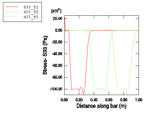
The customized plot appears in Figure 9–8. (For clarity, the default grid and legend positions have been changed.)
We can see that the length of the bar affected by the stress wave is approximately 0.2 m in each of the three curves. This distance should correspond to the distance that the blast wave travels during its time of application, which can be checked by a simple calculation. If the length of the wave front is 0.2 m and the wave speed is 5.15 × 10³ m/s, the time it takes for the wave to travel 0.2 m is 3.88 × 10⁵ s. As expected, this is the duration of the blast load that we applied. The stress wave is not exactly square as it passes along the bar. In particular, there is “ringing” or oscillation of the stress behind the sudden changes in stress. Linear bulk viscosity, discussed later in this chapter, damps the ringing so that it does not affect the results adversely.
Creating a history plot
Another way to study the results is to view the time history of stress at three different points within the bar.
To plot the stress history:
In the Results Tree, click mouse button 3 on History Output and deselect Group Children from the menu that appears.
Select the data for the three elements. Use [Ctrl]+Click to select multiple X–Y data sets.
Click mouse button 3, and select Plot from the menu that appears.
Abaqus/Viewer displays an X–Y plot of the longitudinal stress in each element versus time.
Click ![]() in the prompt area to cancel the current procedure.
in the prompt area to cancel the current procedure.
As before, you can customize the appearance of the plot.
To customize the X–Y plot:
Double-click the X-axis.
The Axis Options dialog box appears.
Switch to the Title tabbed page.
Specify Total time (s) as the X-axis title.
Click Dismiss to close the dialog box.
To customize the appearance of the curves in the X–Y plot:
In the Visualization toolbox, click ![]() to open the Curve Options dialog box.
to open the Curve Options dialog box.
In the Curves field, select the temporary X–Y data label that corresponds to the element closest to the free end of the bar. (Of the elements in this set, this one is affected first by the stress wave.)
Enter S33-0.25 as the curve legend text.
In the Curves field, select the temporary X–Y data label that corresponds to the element in the middle of the bar. (This is the element affected next by the stress wave.)
Specify S33-0.5 as the curve legend text, and change the curve style to dotted.
In the Curves field, select the temporary X–Y data label that corresponds to the element closest to the fixed end of the bar. (This is the element affected last by the stress wave.)
Specify S33-0.75 as the curve legend text, and change the curve style to dashed.
Click Dismiss to close the dialog box.
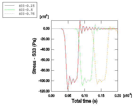
The customized plot appears in Figure 9–9. (For clarity, the default grid and legend positions have been changed.)
In the history plot we can see that stress at a given point increases as the stress wave travels through the point. Once the stress wave has passed completely through the point, the stress at the point oscillates about zero.
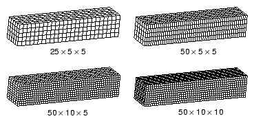
In “Automatic time incrementation and stability,” Section 9.3, we discussed how mesh refinement affects the stability limit and the CPU time. Here we will illustrate this effect with the wave propagation problem. We began with a reasonably refined mesh of square elements with 50 elements along the length and 10 elements in each of the two transverse directions. For illustrative purposes, we will now use a coarse mesh of 25 × 5 × 5 elements and observe how refining the mesh in the various directions changes the CPU time. The four meshes are shown in Figure 9–10.
Table 9–1 shows how the CPU time (normalized with respect to the coarse mesh model result) changes with mesh refinement for this problem. The first half of the table provides the expected results, based on the simplified stability equations presented in this guide; the second half of the table provides the results obtained by running the analyses in Abaqus/Explicit on a desktop workstation.
Table 9–1 Mesh refinement and solution time.
| Mesh | Simplified Theory | Actual | ||||
|---|---|---|---|---|---|---|
| Number of Elements | CPU Time (s) | Max | Number of Elements | Normalized CPU Time | ||
| 25 × 5 × 5 | A | B | C | 5.754E-06 | 625 | 1 |
| 50 × 5 × 5 | A/2 | 2B | 4C | 2.954E-06 | 1250 | 4 |
| 50 × 10 × 5 | A/2 | 4B | 8C | 2.933E-06 | 2500 | 8.33 |
| 50 × 10 × 10 | A/2 | 8B | 16C | 2.907E-06 | 5000 | 16.67 |
For the theoretical results we choose the coarsest mesh, 25 × 5 × 5, as the base state, and we define the stable time increment, the number of elements, and the CPU time as variables A, B, and C, respectively. As the mesh is refined, two things happen: the smallest element dimension decreases, and the number of elements in the mesh increases. Each of these effects increases the CPU time. In the first level of refinement, the 50 × 5 × 5 mesh, the smallest element dimension is cut in half and the number of elements is doubled, increasing the CPU time by a factor of four over the previous mesh. However, further doubling the mesh to 50 × 10 × 5 does not change the smallest element dimension; it only doubles the number of elements. Therefore, the CPU time increases by only a factor of two over the 50 × 5 × 5 mesh. Further refining the mesh so that the elements are uniform and square in the 50 × 10 × 10 mesh again doubles the number of elements and the CPU time.
This simplified calculation predicts quite well the trends of how mesh refinement affects the stable time increment and CPU time. However, there are reasons why we did not compare the predicted and actual stable time increment values. First, recall that we made the approximation that the stable time increment is
![]()
The same wave propagation analysis performed on different materials would take different amounts of CPU time, depending on the wave speed of the material. For example, if we were to change the material from steel to aluminum, the wave speed would change from 5.15 × 10³ m/s to