To demonstrate how to restart an analysis, take the pipe section example in “Example: vibration of a piping system,” Section 11.3, and restart the simulation, adding two additional steps of load history. The first simulation predicted that the piping section would be vulnerable to resonance when extended axially; you must now determine how much additional axial load will increase the pipe's lowest vibrational frequency to an acceptable level.
Step 3 will be a general step that increases the axial load on the pipe to 8 MN, and Step 4 will calculate the eigenmodes and eigenfrequencies again.
Create a new input file, called pipe-2.inp, and add the option blocks discussed below. If you wish to create the entire model using Abaqus/CAE, refer to “Example: restarting the pipe vibration analysis,” Section 11.5 of Getting Started with Abaqus: Interactive Edition.
The only model data required are the *HEADING option and a *RESTART option to read the restart data from the end of the previous analysis. Abaqus reads all other model data, such as node and element definitions, directly from the restart file. Add the following option blocks to your new input file:
*HEADING
Increase tensile load on the piping system
and determine lowest frequency.
*RESTART, READ
Neither the INCREMENT nor the STEP parameter is included on the *RESTART, READ option since by default Abaqus will read the data for the last increment written to the restart file. Since you are continuing the simulation from the end of the previous analysis, no parameters are needed.
The history data consist of two steps. Apply a tensile load (8 MN) to the pipe section in Step 3. The following option block must be placed in Step 3:
*CLOAD
RIGHT, 1, 8.0E6
Set the initial time increment in Step 3 to 1/10 the total step time, which should be 1.0. Step 4 is an exact copy of Step 2 from the previous analysis. All of the load history option blocks necessary to define this restart analysis are shown below.
*STEP, NLGEOM=YES
Apply 8 MN axial tensile load
*STATIC
0.1, 1.
*CLOAD
RIGHT, 1, 8.0E6
*RESTART, WRITE, FREQUENCY=10
*OUTPUT, FIELD, FREQUENCY=10, VARIABLE=PRESELECT
*OUTPUT, HISTORY
*ELEMENT OUTPUT, ELSET=ELEMENT25
S, SINV
*END STEP
*STEP, PERTURBATION
Extract modes and frequencies
*FREQUENCY
8,
*RESTART, WRITE
*OUTPUT, FIELD, VARIABLE=PRESELECT
*END STEP
The complete input file for this restart analysis is listed in “Vibration of a piping system,” Section A.12.
When running a simulation that will need to read data from a restart file, you must specify the root name of the restart file, without the .res extension, with the oldjob parameter on the Abaqus command line. Thus, use the following command to run this restart analysis:
abaqus job=pipe-2 oldjob=pipe
Again, check the status file as the job is running. When the analysis completes, the contents of the status file will look like
 SUMMARY OF JOB INFORMATION:
 STEP  INC ATT SEVERE EQUIL TOTAL  TOTAL      STEP       INC OF       DOF    IF
               DISCON ITERS ITERS  TIME/    TIME/LPF    TIME/LPF    MONITOR RIKS
               ITERS               FREQ
   3     1   1     0     1     1  1.10       0.100      0.1000
   3     2   1     0     1     1  1.20       0.200      0.1000
   3     3   1     0     1     1  1.35       0.350      0.1500
   3     4   1     0     1     1  1.58       0.575      0.2250
   3     5   1     0     1     1  1.91       0.913      0.3375
   3     6   1     0     1     1  2.00       1.00       0.08750
   4     1   1     0     6     0  2.00       1.00e-36   1.000e-36
This analysis starts at Step 3 since Steps 1 and 2 were completed in the previous analysis. There are now two output database (.odb) files associated with this simulation. Data for Steps 1 and 2 are in the file pipe.odb; data for Steps 3 and 4 are in the file pipe-2.odb. When plotting results in Abaqus/Viewer, you need to remember which results are stored in each file, and you need to ensure that Abaqus/Viewer is using the correct output database file.
Start Abaqus/Viewer and specify that the output database file from the restart analysis should be used by giving the following command:
abaqus viewer odb=pipe-2
Plotting the eigenmodes of the pipe
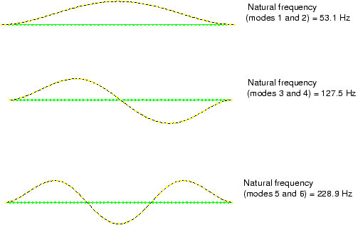
Plot the same six eigenmode shapes of the pipe section for this simulation as were plotted in the previous analysis. The eigenmode shapes can be plotted using the procedures described for the original analysis. These eigenmodes and their natural frequencies are shown in Figure 11–12; again, the corresponding mode shapes lie in planes orthogonal to each other.
Under 8 MN of axial load, the lowest mode is now at 53.1 Hz, which is greater than the required minimum of 50 Hz. If you want to find the exact load at which the lowest mode is just above 50 Hz, you can repeat this restart analysis and change the value of the applied load.
Plotting X–Y graphs from field data for selected steps
Use the field data stored in the output database files, pipe.odb and pipe-2.odb, to plot the history of the axial stress in the pipe for the whole simulation.
To generate a history plot of the axial stress in the pipe for the restart analysis:
In the Results Tree, double-click XYData.
The Create XY Data dialog box appears.
Select ODB field output from this dialog box, and click Continue to proceed.
The XY Data from ODB Field Output dialog box appears.
In the Variables tabbed page of this dialog box, accept the default selection of Integration Point for the variable position and select S11 from the list of available stress components.
At the bottom of the dialog box, toggle Select for the section point and click Settings to choose a section point.
In the Field Report Section Point Settings dialog box that appears, select the category beam and choose any of the available section points for the pipe cross-section. Click OK to exit this dialog box.
In the Elements/Nodes tabbed page of the XY Data from ODB Field Output dialog box, select Element labels as the selection Method. There are 30 elements in the model, and they are numbered consecutively from 1 to 30. Enter any element number (for example, 25) in the Element labels text field that appears on the right side of the dialog box.
Click Active Steps/Frames, and select Step-3 as the only step from which to extract data.
At the bottom of the XY Data from ODB Field Output dialog box, click Plot to see the history of axial stress in the element.
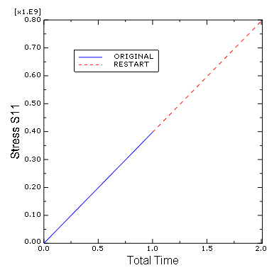
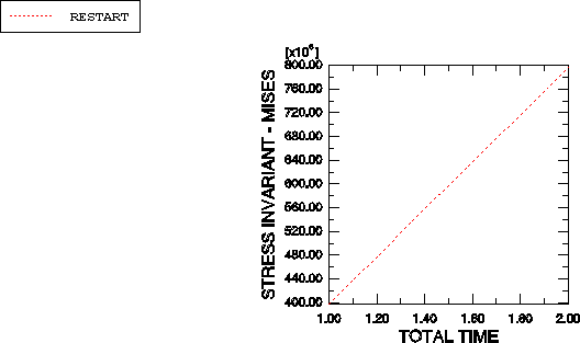
The plot traces the axial stress history at each integration point of the element in the restart analysis. Since the restart is a continuation of an earlier job, it is often useful to view the results from the entire (original and restarted) analysis.
To generate a history plot of the axial stress in the pipe for the entire analysis:
Save the current plot by clicking Save at the bottom of the XY Data from ODB Field Output dialog box. Two curves are saved (one for each integration point), and default names are given to the curves.
Rename either curve RESTART, and delete the other curve.
From the main menu bar, select File![]() Open; or use the
Open; or use the ![]() tool in the File toolbar to open the file pipe.odb.
tool in the File toolbar to open the file pipe.odb.
Following the procedure outlined above, save the plot of the axial stress history for the same element and integration/section point used above. Name this plot ORIGINAL.
In the Results Tree, expand the XYData container.
The ORIGINAL and RESTART curves are listed underneath.
Select both plots with [Ctrl]+Click. Click mouse button 3, and select Plot from the menu that appears to create a plot of axial stress history in the pipe for the entire simulation.
To change the style of the line, open the Curve Options dialog box.
For the RESTART curve, select a dotted line style.
Click Dismiss to close the dialog box.
To change the axis titles, open the Axis Options dialog box.
In this dialog box, switch to the Title tabbed page.
Change the X-axis title to TOTAL TIME, and change the Y-axis title to STRESS S11.
Click Dismiss to close the dialog box.
The plot created by these commands is shown in Figure 11–13. The axial stress history of the same element during Step 3 can be plotted by itself by selecting only the RESTART curve (see Figure 11–14).