Product: Abaqus/CFD
Time accuracy, laminar flow, surface output, time-history data, spatial and temporal accuracy.
Two-dimensional laminar flow over a cylinder is a well-documented fluid dynamics problem, which makes it suitable for verification. This problem is characterized by boundary layer separation resulting from adverse pressure gradients induced by the cylinder geometry. The flow is characterized by a Reynolds number, ![]() , defined with a free-stream velocity, V, and cylinder diameter, D, where
, defined with a free-stream velocity, V, and cylinder diameter, D, where ![]() and
and ![]() are the dynamic viscosity and density of the fluid, respectively. At sufficiently high Reynolds number,
are the dynamic viscosity and density of the fluid, respectively. At sufficiently high Reynolds number, ![]() , the flow becomes unsteady and is characterized by vortices shed from either side of the cylinder in an alternating manner. The resulting downstream wake pattern is known as a Karman vortex street. The frequency at which the vortices are shed is characterized by a nondimensional parameter known as the Strouhal number
, the flow becomes unsteady and is characterized by vortices shed from either side of the cylinder in an alternating manner. The resulting downstream wake pattern is known as a Karman vortex street. The frequency at which the vortices are shed is characterized by a nondimensional parameter known as the Strouhal number ![]() , where f is the vortex shedding frequency. Experimental studies have demonstrated that the Strouhal number is Reynolds number dependent (Roshko, 1954), indicating that, despite the simple geometry, the flow is far from being simple.
, where f is the vortex shedding frequency. Experimental studies have demonstrated that the Strouhal number is Reynolds number dependent (Roshko, 1954), indicating that, despite the simple geometry, the flow is far from being simple.
This problem was selected as an Abaqus/CFD verification problem because of the simple geometry, the unsteady dynamics, and the availability of experimental and numerical results for comparison. Specifically, we consider the case of ![]() flow as the benchmark problem for which the Strouhal number,
flow as the benchmark problem for which the Strouhal number, ![]() , is obtained from the experimental data using the correlation formula given by Roshko, 1954. The objective of the study is to reproduce the unsteady structure of the flow and to measure the convergence rate of Abaqus/CFD.
, is obtained from the experimental data using the correlation formula given by Roshko, 1954. The objective of the study is to reproduce the unsteady structure of the flow and to measure the convergence rate of Abaqus/CFD.
Model:
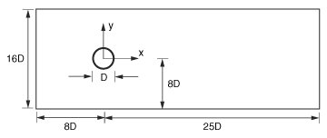
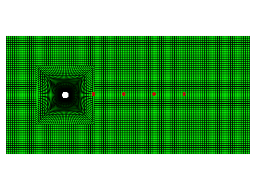
The model consists of a two-dimensional cylinder in a rectangular domain, as shown in Figure 3.3.1–1. The inflow boundary is located 8D upstream of the cylinder axis, the outflow boundary surface is located 25D downstream of the cylinder axis, and the top and bottom surfaces are located 8D away from the cylinder axis. The thickness of the cylinder is 0.2D in the spanwise direction.
Mesh:
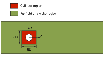
The domain topology (see Figure 3.3.1–2) is partitioned into two regions: the cylinder region—which is the box bounded by ![]() and
and ![]() with the origin located at the center of the cylinder (circle)—and the far field and wake region that cover the complement of the domain.
with the origin located at the center of the cylinder (circle)—and the far field and wake region that cover the complement of the domain.
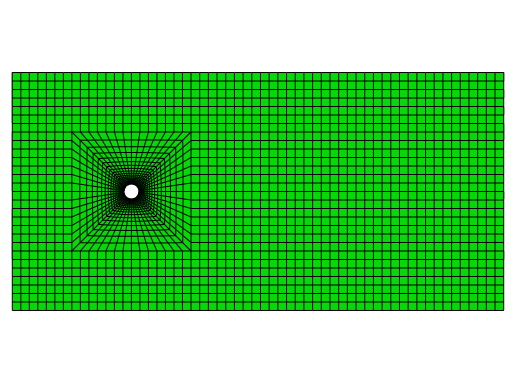
In this study five meshes with varying element sizes, summarized in Table 3.3.1–1, are employed. Mesh refinement is performed uniformly all over the computational domain (see Figure 3.3.1–3). To measure the mesh refinement, a mesh metric h (from ASME V V 20-2009) is used to compare results among meshes:
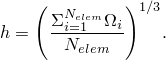
Table 3.3.1–1 Mesh description.
| Mesh | Number of elements | h/D |
|---|---|---|
| 1 | 2,520 | 0.3471 |
| 2 | 4,068 | 0.2959 |
| 3 | 5,902 | 0.2614 |
| 4 | 7,630 | 0.2399 |
| 5 | 10,080 | 0.2187 |
Boundary conditions:
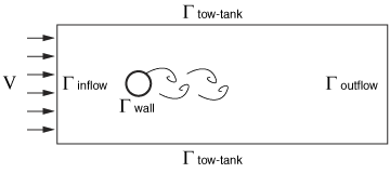
The boundary conditions applied to the model are shown schematically in Figure 3.3.1–4.
At the inflow surface (Initial conditions:
The velocity, V, is set to zero everywhere in the flow domain. Velocity initial conditions that satisfy the solvability conditions for the incompressible Navier-Stokes equations are obtained by inserting the boundary conditions in the prescribed initial velocity field, followed by a projection to a divergence-free subspace. This mass adjustment to the velocity initial conditions is necessary to guarantee that the flow problem is well posed.
Problem setup:
The fluid density, cylinder diameter, inflow velocity, and dynamic viscosity values are specified as ![]() = 1 kg /m3, D = 1 m, V = 1 m/s, and
= 1 kg /m3, D = 1 m, V = 1 m/s, and ![]() = 0.01 kg/ms, respectively. These values yield a Reynolds number of 100. Transient flow simulations using a fixed step size of
= 0.01 kg/ms, respectively. These values yield a Reynolds number of 100. Transient flow simulations using a fixed step size of ![]() and total simulated time t = 350 s are conducted for all meshes. The fixed
and total simulated time t = 350 s are conducted for all meshes. The fixed ![]() used is smaller than the
used is smaller than the ![]() computed using a fixed
computed using a fixed ![]() number for all meshes. A time weight of
number for all meshes. A time weight of ![]() is used for the diffusion and advective terms; and the solver options are set to the defaults with the exception of the pressure Poisson equation (PPE) solver tolerance, which is set to 108 (default 105).
is used for the diffusion and advective terms; and the solver options are set to the defaults with the exception of the pressure Poisson equation (PPE) solver tolerance, which is set to 108 (default 105).
This verification study is intended to assess the time accuracy of Abaqus/CFD for a ![]() flow where a Hopf bifurcation results in steady, periodic vortex shedding. Experimental data and well-established numerical calculations are used as benchmark solutions to compare with the results obtained here.
flow where a Hopf bifurcation results in steady, periodic vortex shedding. Experimental data and well-established numerical calculations are used as benchmark solutions to compare with the results obtained here.
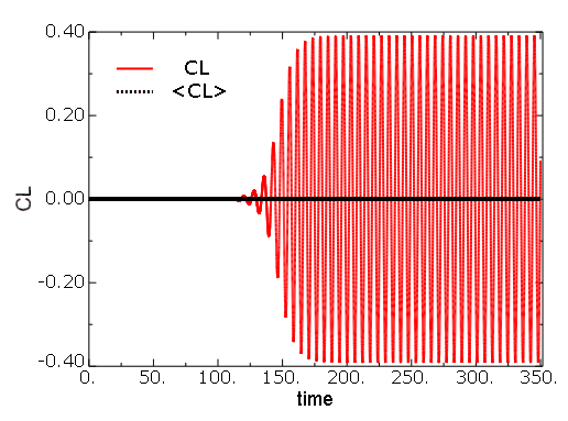
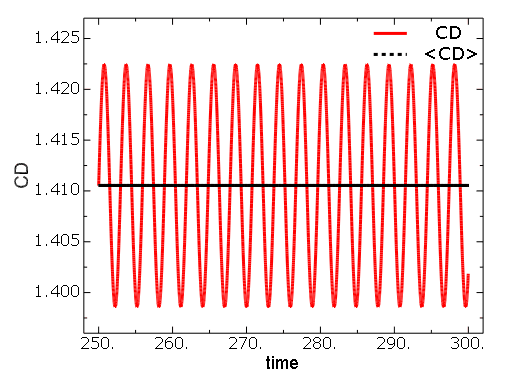
The time at which vortex shedding first develops depends on the mesh quality. For all meshes used in this study, a periodic vortex shedding system is fully established around 225 time units, after which numerical calculations were conducted for a period of 125 time units to collect time-history data for the drag coefficient (![]() ), the lift coefficient (
), the lift coefficient (![]() ), and the velocity (
), and the velocity (![]() ) for all meshes. The
) for all meshes. The ![]() time history signals were analyzed using a numerical discrete Fast Fourier Transform to extract the dominant frequency. For this moderate
time history signals were analyzed using a numerical discrete Fast Fourier Transform to extract the dominant frequency. For this moderate ![]() case there is only one dominant frequency (corresponding to the Hopf bifurcation) that can also be computed directly by counting the number of zero crossings during the time sample. Both approaches yielded effectively the same results.
case there is only one dominant frequency (corresponding to the Hopf bifurcation) that can also be computed directly by counting the number of zero crossings during the time sample. Both approaches yielded effectively the same results.
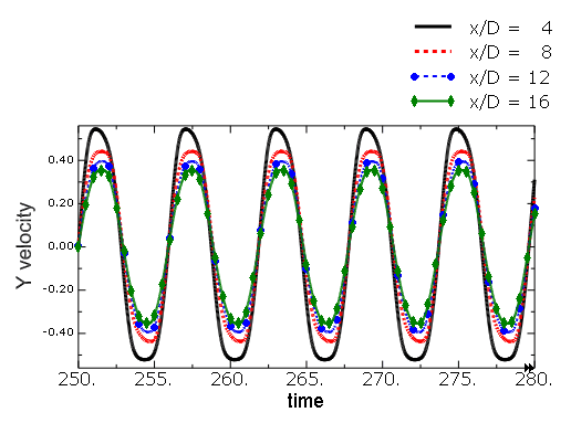
Figure 3.3.1–5 indicates the four locations, ![]() = (4, 8, 12, 16) approximately, and
= (4, 8, 12, 16) approximately, and ![]() above the centerline, marked in red, where the time history of y-velocity is collected for Mesh 5.
above the centerline, marked in red, where the time history of y-velocity is collected for Mesh 5.
![]()
![]()
Following the same procedure, the Strouhal numbers computed for all meshes employed in this study are summarized in Table 3.3.1–2.
Table 3.3.1–2 Calculated Strouhal number.
| Mesh | Number of samples per period | ||
|---|---|---|---|
| 1 | 0.01 | 0.1559 | 641 |
| 2 | 0.01 | 0.1639 | 610 |
| 3 | 0.01 | 0.1639 | 610 |
| 4 | 0.01 | 0.1679 | 600 |
| 5 | 0.01 | 0.1679 | 600 |
Table 3.3.1–3 Calculated Strouhal number from benchmark calculations (Engelman and Jamnia, 1990).
| Mesh | Number of samples per period | ||
|---|---|---|---|
| Coarse | 0.269 | 0.172 | 22 |
| Medium | 0.264 | 0.172 | 22 |
| Fine | 0.266 | 0.173 | 22 |
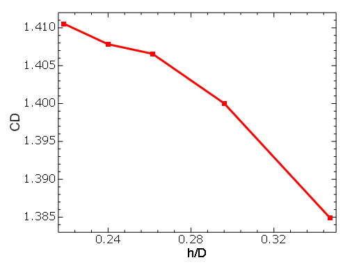
To further assess the spatial accuracy of the code, the mean drag coefficient obtained by averaging the ![]() time signal is used with a Richardson extrapolation to estimate the convergence rate. Results are summarized in Table 3.3.1–4, and Figure 3.3.1–10 shows the convergence of the drag coefficient as a function of the mesh metric (h) . In addition, the benchmark solution taken from Engelman and Jamnia, 1990 is presented in Table 3.3.1–5.
time signal is used with a Richardson extrapolation to estimate the convergence rate. Results are summarized in Table 3.3.1–4, and Figure 3.3.1–10 shows the convergence of the drag coefficient as a function of the mesh metric (h) . In addition, the benchmark solution taken from Engelman and Jamnia, 1990 is presented in Table 3.3.1–5.
Table 3.3.1–4 Calculated mean drag coefficient.
| Mesh | h/D | |
|---|---|---|
| 1 | 0.3471 | 1.3848 |
| 2 | 0.2959 | 1.4000 |
| 3 | 0.2614 | 1.4065 |
| 4 | 0.2399 | 1.4078 |
| 5 | 0.2187 | 1.4105 |
Table 3.3.1–5 Calculated mean drag coefficient from benchmark calculations (Engelman and Jamnia, 1990).
| Mesh | h/D | |
|---|---|---|
| Coarse | 0.7791 | 1.405 |
| Medium | 0.6930 | 1.410 |
| Fine | 0.6128 | 1.411 |
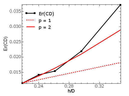
The rate of spatial convergence of Abaqus/CFD can be estimated using the results of the four meshes. Following ASME V V 20-2009, the error in the numerical solution can be computed as
![]()
![]()
Following ASME V V 20-2009, the observed convergence between two calculations can be approximated as
![]()
The unsteady incompressible flow over a cylinder was successfully computed using Abaqus/CFD. The vortex shedding frequencies computed were found to be in good agreement with the experimental data and previous numerical calculations. Furthermore, the estimated overall convergence rate for the Abaqus/CFD drag coefficient was measured and was found to be in close agreement with the theoretical second-order accuracy of the code.
Mesh 1: Mesh with 2520 elements.
Mesh 2: Mesh with 4068 elements.
Mesh 3: Mesh with 5902 elements.
Mesh 4: Mesh with 7630 elements.
Mesh 5: Mesh with 10080 elements.
ASME V V 20-2009, “Standard for Verification and Validation in Computational Fluid Dynamics and Heat Transfer,” American Society of Mechanical Engineers.
Engelman, M. S., and M. A. Jamnia, “Transient Flow Past a Circular Cylinder: A Benchmark Solution,” International Journal for Numerical Methods in Fluids, vol. 11, pp. 985–1000, 1990.
Roshko, A., “On the Development of Turbulent Wakes from Vortex Streets,” National Advisory Committee for Aeronautics, Washington, D. C., Report 1191, 1954.
Wieselsberger, C., “New Data on the Laws of Fluid Resistance,” NACA-TN-84, 1922.