Product: Abaqus/CFD
Outflow boundary conditions, implicit advection, and Incomplete Lower Upper decomposition (LU) factorization preconditioned Flexible Generalized Minimal Residual (FGMRES) method for momentum transport.
The problem of steady viscous isothermal incompressible flow over a backward-facing step is a canonical computational fluid dynamics test problem that has been used by numerous researchers to assess a broad variety of solution methods. This flow problem exercises the ability of a solution method to handle massive separation behind the step, followed by reattachment of a laminar boundary layer, while providing an essentially passive outflow boundary condition that does not disturb the primary physical features of the flow problem. In addition, the presence of a pressure singularity at the corner of the step presents a challenging problem in terms of the efficiency of the pressure solution strategy.
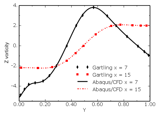
In this verification exercise the problem definition presented by Gartling (1990) is used to define the geometry and associated boundary conditions for a ![]() = 800 flow. The flow domain as described by Gartling (1990) is shown in Figure 3.3.4–1. A series of five meshes with increasing mesh resolution are used to compute the flow fields in this study. The primary separation and reattachment points along the top and bottom walls of the flow domain are compared to published data. In addition, velocity, pressure, and vorticity distributions are compared with the benchmark results of Gartling (1990).
= 800 flow. The flow domain as described by Gartling (1990) is shown in Figure 3.3.4–1. A series of five meshes with increasing mesh resolution are used to compute the flow fields in this study. The primary separation and reattachment points along the top and bottom walls of the flow domain are compared to published data. In addition, velocity, pressure, and vorticity distributions are compared with the benchmark results of Gartling (1990).
Model:
The backward-facing step model consists of a planar domain with a channel height H, step height ![]() , and overall channel length of 30 H or 60 step heights from the inlet. Since the two-dimensional problem is solved as an abstraction of the three-dimensional version, an out-of-plane thickness equal to
, and overall channel length of 30 H or 60 step heights from the inlet. Since the two-dimensional problem is solved as an abstraction of the three-dimensional version, an out-of-plane thickness equal to ![]() is used.
is used.
Mesh:
The mesh design for the backward-facing step followed the suggestions in Gartling (1990) and Christon (1997). The rectangular channel is divided into two distinct regions, an upstream section and a downstream section. The upstream section uses a uniform mesh in the region ![]() , and the downstream section in the region
, and the downstream section in the region ![]() is smoothly graded in the flow direction so that the elements at the outflow boundary are approximately twice the size of those at the inlet to the channel.
is smoothly graded in the flow direction so that the elements at the outflow boundary are approximately twice the size of those at the inlet to the channel.
The mesh characteristics for each of the five meshes are shown in Table 3.3.4–1. Here, the element size refers to the mesh spacing in the uniform upstream region of the mesh where ![]() .
.
Table 3.3.4–1 Characteristic meshes used in the present study.
| Mesh | Number of Elements | Element Size |
|---|---|---|
| A | 8000 | 0.06 |
| B | 32000 | 0.03 |
| C | 72000 | 0.020 |
| D | 128000 | 0.015 |
| E | 512000 | 0.0075 |
Boundary conditions:
The prescribed boundary conditions for the backward-facing step problem include the no-slip/no-penetration conditions at the channel walls, as shown in Figure 3.3.4–1. At the inlet the velocity field is assumed to be hydrodynamically fully developed with a parabolic profile in the horizontal velocity component; i.e., ![]() . This velocity profile yields an average horizontal velocity of
. This velocity profile yields an average horizontal velocity of ![]() and a maximum of
and a maximum of ![]() . The two-dimensional nature of the flow problem requires that the z-velocity be prescribed as
. The two-dimensional nature of the flow problem requires that the z-velocity be prescribed as ![]() on the front/back planes of the flow domain. At the outflow the flow is assumed to be parallel with a zero stress condition; i.e.,
on the front/back planes of the flow domain. At the outflow the flow is assumed to be parallel with a zero stress condition; i.e., ![]() . The “do-nothing” boundary conditions on the x-momentum transport equation automatically force the shear term to be zero, while the outflow pressure is prescribed to be zero at the outflow boundary.
. The “do-nothing” boundary conditions on the x-momentum transport equation automatically force the shear term to be zero, while the outflow pressure is prescribed to be zero at the outflow boundary.
Initial conditions:
At t = 0, the velocity is set to zero everywhere in the flow domain. To guarantee a well-posed incompressible Navier-Stokes problem, the prescribed boundary conditions are inserted into the initial conditions, which are projected onto a divergence-free subspace. Such a projection ensures that the initial velocity field satisfies the prescribed boundary conditions and is also divergence free. Subsequent to the initial velocity adjustment, initial pressures that are consistent with the divergence-free initial velocity are computed.
Problem setup:
The following values are used for the flow problem: the fluid density is ![]() = 1 kg/m3, the fluid viscosity is
= 1 kg/m3, the fluid viscosity is ![]() = 1.25 × 10³ kg/m
= 1.25 × 10³ kg/m ![]() s, the channel height is
s, the channel height is ![]() , and the average inflow velocity is
, and the average inflow velocity is ![]() . The Reynolds number is defined as
. The Reynolds number is defined as ![]() so that
so that ![]() for these parameters.
for these parameters.
To allow the problem to reach a steady-state condition rapidly, all calculations presented below use a time weight of ![]() for the advective and viscous terms; i.e., advection is treated implicitly. This choice corresponds to a backward Euler time integration method. The convergence criteria for the pressure is specified as
for the advective and viscous terms; i.e., advection is treated implicitly. This choice corresponds to a backward Euler time integration method. The convergence criteria for the pressure is specified as ![]() = 1.0 ×10⁸. The momentum transport solver is specified as FGMRES with ILU preconditioning. The time incrementation options specify the Courant-Friedrichs-Lewy (CFL) stability condition equal to 40 and a termination time of 400 time units. No maximum time step limit is imposed. All other solver options use default values.
= 1.0 ×10⁸. The momentum transport solver is specified as FGMRES with ILU preconditioning. The time incrementation options specify the Courant-Friedrichs-Lewy (CFL) stability condition equal to 40 and a termination time of 400 time units. No maximum time step limit is imposed. All other solver options use default values.
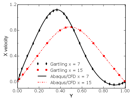
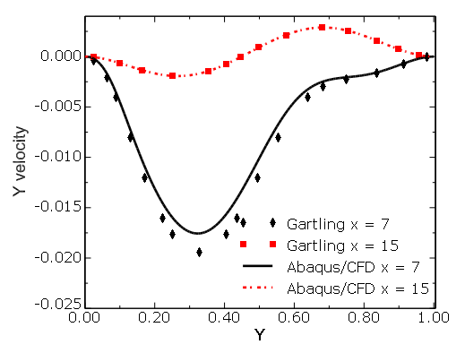
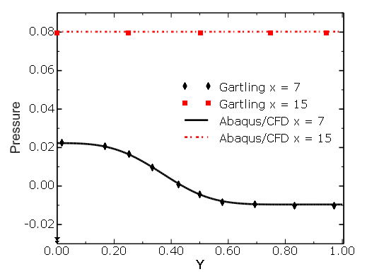
For comparison with published results of the Re = 800 backward-facing step problem, the separation/reattachment lengths are evaluated. In addition, the pressure, velocity, and vorticity profiles in the streamwise and cross-flow directions are compared with the published benchmark data of Gartling (1990). This verification study is performed using a series of five meshes with increasing mesh resolution.
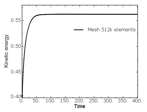
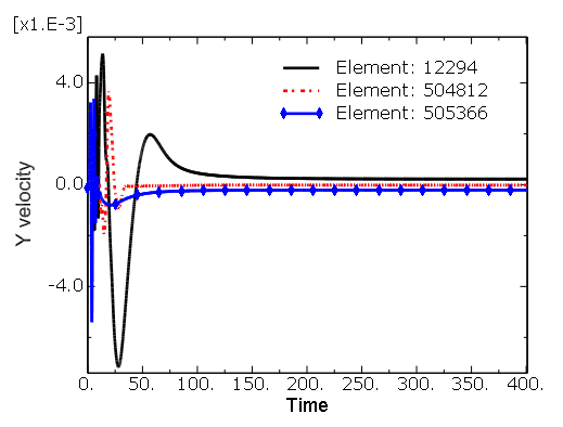
For each calculation on each mesh, time-history data of the horizontal and vertical velocity components, in addition to the global kinetic energy, are examined. The velocity and kinetic energy time histories reach stationary values by the termination time of 400 time units, indicating that a valid steady-state solution is achieved for each mesh. Preliminary tests are performed varying the CFL number from 1 to 40. Identical results are obtained at each CFL number, indicating that the solution is not sensitive to the time incrementation size. Figure 3.3.4–2 shows the horizontal velocity time histories, and Figure 3.3.4–3 shows the vertical velocity time histories at three points downstream of the step for mesh E. Element 12294 is located at (3.7988,0.4781,0.05), 504812 at (5.9138, 0.4844, 0.05), and 505366 at (1.7588, 0.4844, 0.05). The global kinetic energy time history is shown in Figure 3.3.4–4 for mesh E.
Figure 3.3.4–2 Time history of the horizontal velocity at locations downstream of the step for mesh E with 512,000 elements.
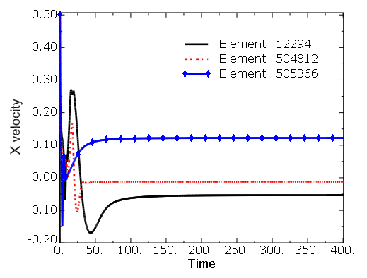
Figure 3.3.4–3 Time history of the vertical velocity at locations downstream of the step for mesh E with 512,000 elements.
The primary separation and reattachment lengths are presented in Table 3.3.4–2. Here, ![]() is the length from the step face to the downstream reattachment point at the bottom of the channel. On the upper wall of the channel,
is the length from the step face to the downstream reattachment point at the bottom of the channel. On the upper wall of the channel, ![]() marks the first separation point measured from the inlet to the channel, and
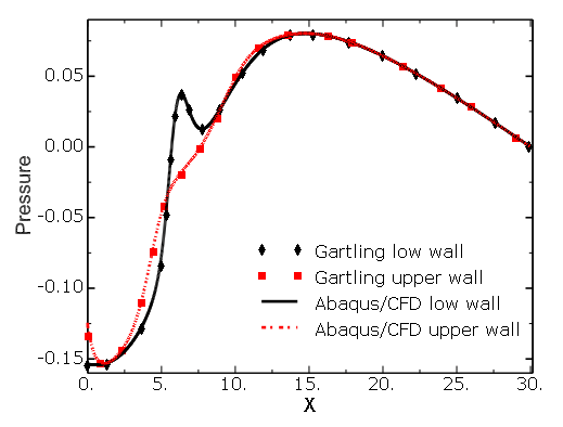
marks the first separation point measured from the inlet to the channel, and ![]() locates the reattachment point also measured from the inlet to the channel. In comparison to the benchmark results provided by Gartling (1990) and the results by Christon (1997), the computed separation and reattachment lengths show very good agreement. The results for the coarsest mesh, mesh A, indicate that the flow field is quite under resolved using only 8,000 elements. The mesh resolution used by Gartling (1990) with biquadratic velocity and discontinuous linear pressure approximation corresponds only approximately to the resolution used by Christon (1997) with a bilinear velocity and discontinuous pressure approximation. In constrast, mesh D provides somewhat fewer velocity degrees of freedom relative to the 128,000 element mesh used by Christon (1997), while mesh E provides slightly more velocity degrees of freedom. The errors between the mesh E results and those of Gartling (1990) are less than 1%.
locates the reattachment point also measured from the inlet to the channel. In comparison to the benchmark results provided by Gartling (1990) and the results by Christon (1997), the computed separation and reattachment lengths show very good agreement. The results for the coarsest mesh, mesh A, indicate that the flow field is quite under resolved using only 8,000 elements. The mesh resolution used by Gartling (1990) with biquadratic velocity and discontinuous linear pressure approximation corresponds only approximately to the resolution used by Christon (1997) with a bilinear velocity and discontinuous pressure approximation. In constrast, mesh D provides somewhat fewer velocity degrees of freedom relative to the 128,000 element mesh used by Christon (1997), while mesh E provides slightly more velocity degrees of freedom. The errors between the mesh E results and those of Gartling (1990) are less than 1%.
Table 3.3.4–2 Primary separation and reattachment lengths for the backward-facing step problem.
| Mesh | Lower Reattachment ( | Upper Separation ( | Upper Reattachment ( |
|---|---|---|---|
| A | 4.47 | 3.89 | 8.93 |
| B | 5.67 | 4.76 | 10.06 |
| C | 5.89 | 4.87 | 10.24 |
| D | 5.97 | 4.89 | 10.32 |
| E | 6.06 | 4.90 | 10.41 |
| Gartling | 6.10 | 4.85 | 10.48 |
| Christon | 6.03 | 4.90 | 10.37 |
Figure 3.3.4–5 shows pressure contours in the channel in the region just downstream of the step.
Figure 3.3.4–5 Pressure contours for mesh E. Contour levels are –0.1757, –0.1657, –0.1557, –0.1457, –0.1357, –0.1257, –0.1157, –0.1057, –0.0957, –0.0857, –0.0757, –0.0557, –0.0357, –0.0157, 0.0043, 0.0243, 0.0443, 0.0643.

Figure 3.3.4–6 Vorticity contours for mesh E. Contour levels are 10.0, 8.0, 4.0, 2.0, 0.0, –2.0, –4.0, –6.0, –8.0.
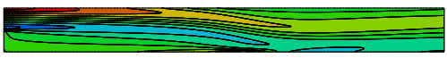
Figure 3.3.4–7 Fluid speed contours for mesh E. Contour levels are 0.05, 0.10, 0.15, 0.20, 0.40, 0.60, 0.80, 1.0, 1.20, 1.40.
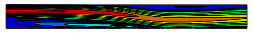
Figure 3.3.4–8 shows the pressure distribution along the upper and lower walls of the channel relative to results presented by Gartling (1990).
Figure 3.3.4–8 Pressure distribution in the streamwise direction along the top and bottom walls of the channel.
A series of five meshes are used for the calculation of laminar flow over a backward-facing step at Re = 800. Implicit advection with a fixed CFL = 40 and a backward Euler time integration are used to achieve a steady-state flow condition at 400 time units. A direct and detailed comparison of the results produced with Abaqus/CFD and published benchmark data demonstrates excellent agreement.
Backward-facing step with 8,000 elements.
Backward-facing step with 32,000 elements.
Backward-facing step with 72,000 elements.
Backward-facing step with 128,000 elements.
Backward-facing step with 512,000 elements.
Christon, M. A., “A Domain-Decomposition Message-Passing Approach to Transient Viscous Incompressible Flow Using Explicit Time Integration,” Computer Methods in Applied Mechanics and Engineering, vol. 148, pp. 329–352, 1997.
Gartling, D. K., “A Test Problem for Outflow Boundary Conditions—Flow over a Backward-Facing Step,” International Journal for Numerical Methods in Fluids, vol. 11, pp. 953–967, 1990.