Product: Abaqus/CFD
The continuity and the Brinkman-Forchheimer equations governing the flow of an incompressible fluid in a fluid-saturated porous media can be written as follows (Nield and Bejan, 2010):
![]()
![]()
Thus, the porous media flow problem requires the specification of the porosity ![]() and the permeability
and the permeability ![]() of the porous medium. The default value of
of the porous medium. The default value of ![]() ( = 0.142887) can also be changed in the material property definition. For the case of turbulent flow within a porous medium, the fluid viscosity
( = 0.142887) can also be changed in the material property definition. For the case of turbulent flow within a porous medium, the fluid viscosity ![]() includes the contribution of both the molecular and the turbulent eddy viscosities.
includes the contribution of both the molecular and the turbulent eddy viscosities.
If we define a length scale ![]() , a velocity scale
, a velocity scale ![]() , and a time scale
, and a time scale ![]() , the above governing equations can be cast in a nondimensional form:
, the above governing equations can be cast in a nondimensional form:
![]()
![]()
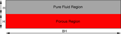
This verification problem is used to evaluate the accuracy of the Abaqus/CFD porous media model for the case of a porous interface placed parallel to the flow direction. The geometry consists of a channel partially filled with a horizontal layer of porous medium, as shown in Figure 3.3.5–1. Steady flow is considered for the following two cases: ![]() ,
, ![]() ; and
; and ![]() ,
, ![]() . The Reynolds number is based on the average outflow velocity of the pure fluid region (see Figure 3.3.5–1) under fully developed conditions and the height, H, of the porous medium. Two values of
. The Reynolds number is based on the average outflow velocity of the pure fluid region (see Figure 3.3.5–1) under fully developed conditions and the height, H, of the porous medium. Two values of ![]() equal to
equal to ![]() and
and ![]() are used for the present problem and are based on H. The results provided by Betchen et al. (2006), are used as the reference solution. The value of the porosity,
are used for the present problem and are based on H. The results provided by Betchen et al. (2006), are used as the reference solution. The value of the porosity, ![]() , is set to 0.7 for all the cases.
, is set to 0.7 for all the cases.
Model:
The geometry of the two-dimensional problem is shown in Figure 3.3.5–1. The height of the pure fluid domain is given by H, which is set equal to that of the porous medium. The length of the channel is set equal to 8H. Since the two-dimensional problem is solved as an abstraction of the three-dimensional version, an out-of-plane thickness equal to 0.2H is specified.
Mesh:
For both values of Da, a mesh sensitivity study was performed by comparing the value of the axial velocity at the interface between the porous and pure fluid region across a cross-section of the channel where fully developed flow conditions exist (near the outlet of the domain). Based on the analysis, the following conclusion was drawn:
For both the cases of ![]() and
and ![]() , a 100 × 40 mesh (length × height) was found to be sufficient to obtain mesh independent results.
, a 100 × 40 mesh (length × height) was found to be sufficient to obtain mesh independent results.
Boundary conditions:
At the inlet a constant horizontal velocity, ![]() , is specified. An outflow boundary condition with the pressure
, is specified. An outflow boundary condition with the pressure ![]() is prescribed at the outflow boundary. A no-slip/no-penetration boundary condition is prescribed at the lower and upper walls. Furthermore, the two-dimensional nature of the problem is enforced by specifying the z-velocity component to be zero at all the boundaries of the domain. The summary of the prescribed boundary conditions is given in Table 3.3.5–1.
is prescribed at the outflow boundary. A no-slip/no-penetration boundary condition is prescribed at the lower and upper walls. Furthermore, the two-dimensional nature of the problem is enforced by specifying the z-velocity component to be zero at all the boundaries of the domain. The summary of the prescribed boundary conditions is given in Table 3.3.5–1.
Table 3.3.5–1 Boundary conditions for the porous channel problem.
| Surface | Boundary Condition |
|---|---|
| Inlet | |
| Outlet | Outflow boundary conditions with p = 0 |
| Top and bottom walls | No-slip/no-penetration |
Initial conditions:
At ![]() , the velocity components are set to zero everywhere in the flow domain.
, the velocity components are set to zero everywhere in the flow domain.
Problem setup:
The following values are used for the flow problem: fluid density ![]() = 1 kg/m3 and height of the pure fluid and porous domains
= 1 kg/m3 and height of the pure fluid and porous domains ![]() = 1 m. The latter implies that the permeability
= 1 m. The latter implies that the permeability ![]() , and the values of K are set accordingly. At the inlet a constant horizontal velocity
, and the values of K are set accordingly. At the inlet a constant horizontal velocity ![]() is determined a priori such that the average outflow velocity for the pure fluid region is equal to 1. For the porous region,
is determined a priori such that the average outflow velocity for the pure fluid region is equal to 1. For the porous region, ![]() = 0.7.
= 0.7.
To achieve a steady state, a backward Euler time integration scheme (the time weights ![]() for all the discretized terms) is used with the implicit advection scheme and the Courant-Friedrichs-Lewy (CFL) number set to 40. All other solver options are set to the default values. Various smaller CFL numbers down to 0.45 were also tested with both the backward Euler and the Crank-Nicolson time integration schemes and with an explicit advection scheme. The steady-state solutions were found to be invariant with respect to these settings.
for all the discretized terms) is used with the implicit advection scheme and the Courant-Friedrichs-Lewy (CFL) number set to 40. All other solver options are set to the default values. Various smaller CFL numbers down to 0.45 were also tested with both the backward Euler and the Crank-Nicolson time integration schemes and with an explicit advection scheme. The steady-state solutions were found to be invariant with respect to these settings.
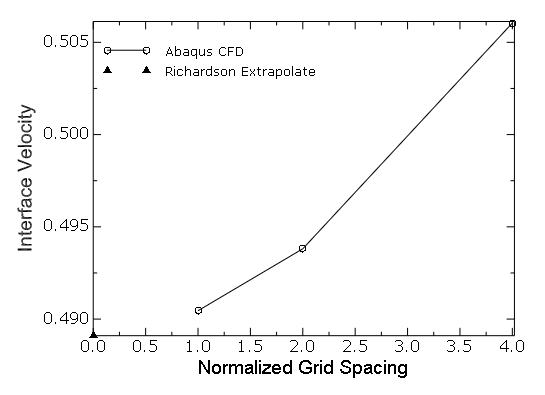
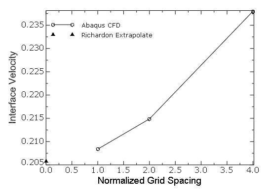
A grid sensitivity study using the Richardson extrapolation procedure was also done on three successively refined meshes with a refinement ratio of 2: a 50 × 20 mesh, a 100 × 40 mesh, and a 200 × 80 mesh. The axial component of the nodal velocity at the interface between the pure fluid and porous media was chosen for the grid convergence study. In addition, the two fine grids were used to estimate the value of the interface velocity at zero-grid spacing (Richardson extrapolate). Figure 3.3.5–2 and Figure 3.3.5–3 show the plots of the interface velocities with varying (normalized) grid spacings for the cases of ![]() and
and ![]() , respectively. The zero-grid spacing Richardson extrapolate is also indicated. The normalization is done by the spacing of the finest grid. As the grid spacing reduces, the interface velocities approach the asymptotic zero-grid spacing values. The orders of convergence observed from these results were also determined to be 1.866 for the case of
, respectively. The zero-grid spacing Richardson extrapolate is also indicated. The normalization is done by the spacing of the finest grid. As the grid spacing reduces, the interface velocities approach the asymptotic zero-grid spacing values. The orders of convergence observed from these results were also determined to be 1.866 for the case of ![]() and 1.832 for the case of
and 1.832 for the case of ![]() . The theoretical order of convergence is 2.0, and the differences can be attributed to the nonlinearities in the problem.
. The theoretical order of convergence is 2.0, and the differences can be attributed to the nonlinearities in the problem.
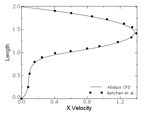
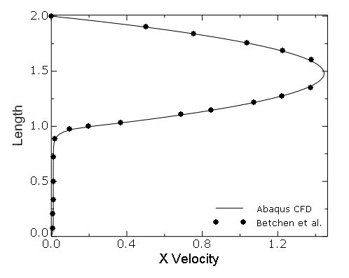
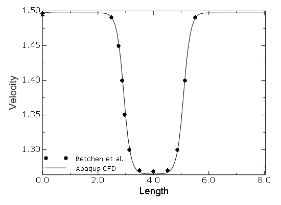
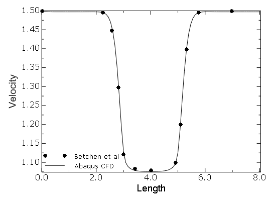
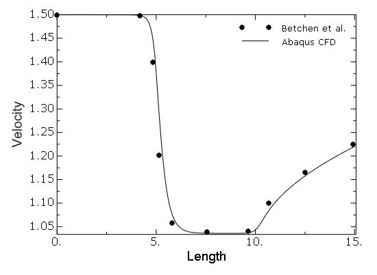
The results of all the cases generated using Abaqus/CFD are compared with the published results of Betchen et al. (2006). In Figure 3.3.5–4 and Figure 3.3.5–5 the axial component of the velocity under fully developed flow conditions existing near the outlet boundary (the specific location was chosen to be at x = 7.84) are plotted for the cases of Da = ![]() and
and ![]() . The results are seen to be in good agreement with the published results. However, in Betchen et al. (2006), only a first-order accurate upwind scheme is used for the advection terms, while Abaqus/CFD uses an advection scheme that is spatially second-order accurate for smoothly varying flows.
. The results are seen to be in good agreement with the published results. However, in Betchen et al. (2006), only a first-order accurate upwind scheme is used for the advection terms, while Abaqus/CFD uses an advection scheme that is spatially second-order accurate for smoothly varying flows.
Porous channel: ![]() ,
, ![]() with a 50 × 20 mesh (length × height).
with a 50 × 20 mesh (length × height).
Porous channel: ![]() ,
, ![]() with a 100 × 40 mesh (length × height).
with a 100 × 40 mesh (length × height).
Porous channel: ![]() ,
, ![]() with a 200 × 80 mesh (length × height).
with a 200 × 80 mesh (length × height).
Porous channel: ![]() ,
, ![]() with a 50 × 20 mesh (length × height).
with a 50 × 20 mesh (length × height).
Porous channel: ![]() ,
, ![]() with a 100 × 40 mesh (length × height).
with a 100 × 40 mesh (length × height).
Porous channel: ![]() ,
, ![]() with a 200 × 80 mesh (length × height).
with a 200 × 80 mesh (length × height).
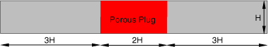
This verification problem is used to evaluate the accuracy of the Abaqus/CFD porous media model for the case of a porous interface placed perpendicular to the flow direction. The geometry consists of a channel partially filled with a porous plug, as shown in Figure 3.3.5–6 and Figure 3.3.5–7.
Steady flow solutions are considered for the following three cases:Model:
For ![]() , the length of the channel is set equal to 8H. As shown in Figure 3.3.5–6, a porous plug of length 2
, the length of the channel is set equal to 8H. As shown in Figure 3.3.5–6, a porous plug of length 2![]() is placed starting at a distance of 3H from the inlet. For the case of
is placed starting at a distance of 3H from the inlet. For the case of ![]() , the channel length is 60H. As shown in Figure 3.3.5–7, a porous plug of length 5H is placed at a distance of 5H from the inlet. The two-dimensional problem is solved as an abstraction of the three-dimensional version, so an out-of-plane thickness equal to 0.2H is specified.
, the channel length is 60H. As shown in Figure 3.3.5–7, a porous plug of length 5H is placed at a distance of 5H from the inlet. The two-dimensional problem is solved as an abstraction of the three-dimensional version, so an out-of-plane thickness equal to 0.2H is specified.
Mesh:
A mesh sensitivity study was performed for all cases based on the comparison of the axial centerline velocity profile at steady-state conditions. The following conclusions were drawn:
For the case of ![]() , a 100 × 40 mesh (length × height) was found to be sufficient to obtain mesh independent results for both
, a 100 × 40 mesh (length × height) was found to be sufficient to obtain mesh independent results for both ![]() and
and ![]() .
.
For the case of ![]() , a 200 × 80 mesh was necessary to obtain mesh independent results.
, a 200 × 80 mesh was necessary to obtain mesh independent results.
Boundary conditions:
At the inlet a fully developed parabolic velocity profile with a mean velocity, ![]() , is prescribed. An outflow boundary condition with the pressure
, is prescribed. An outflow boundary condition with the pressure ![]() is prescribed at the channel outlet. No-slip/no-penetration boundary conditions are prescribed at the lower and upper walls. Furthermore, the two-dimensional nature of the problem is enforced by specifying the z-velocity component to zero everywhere in the domain. The summary of the boundary conditions is given in Table 3.3.5–2.
is prescribed at the channel outlet. No-slip/no-penetration boundary conditions are prescribed at the lower and upper walls. Furthermore, the two-dimensional nature of the problem is enforced by specifying the z-velocity component to zero everywhere in the domain. The summary of the boundary conditions is given in Table 3.3.5–2.
Table 3.3.5–2 Boundary conditions for the porous plug problem. ![]() for all the cases.
for all the cases.
| Surface | Boundary Condition |
|---|---|
| Inlet | |
| Outlet | Outflow boundary condition with |
| Top and bottom walls | No-slip/no-penetration |
Initial conditions:
At ![]() , the velocity components are set to zero everywhere in the flow domain.
, the velocity components are set to zero everywhere in the flow domain.
Problem setup:
The channel height H = 1 m, and the inlet mean velocity ![]() = 1 m/s. To vary the Reynolds number, the density
= 1 m/s. To vary the Reynolds number, the density ![]() and the dynamic viscosity
and the dynamic viscosity ![]() are changed as given in Table 3.3.5–3. Since H = 1, the permeability
are changed as given in Table 3.3.5–3. Since H = 1, the permeability ![]() and the values of K are set accordingly.
and the values of K are set accordingly.
Table 3.3.5–3 Values of the density ![]() and the dynamic viscosity
and the dynamic viscosity ![]() used for the various Re cases.
used for the various Re cases.
| Re | ||
|---|---|---|
| 1 | 1 | 1 |
| 1000 | 0.4 | 0.02 |
To achieve a steady state, use a backward Euler time integration scheme (the time weights ![]() for all the discretized terms) with the implicit advection scheme and the CFL number set to 40. All other solver options are set to the default values. Various smaller CFL numbers down to 0.45 were also tested with both the backward Euler and the Crank-Nicolson time integration schemes and with an explicit advection scheme. The steady-state solutions were found to be invariant with respect to these settings.
for all the discretized terms) with the implicit advection scheme and the CFL number set to 40. All other solver options are set to the default values. Various smaller CFL numbers down to 0.45 were also tested with both the backward Euler and the Crank-Nicolson time integration schemes and with an explicit advection scheme. The steady-state solutions were found to be invariant with respect to these settings.
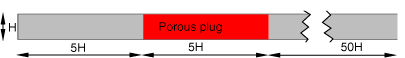
A grid sensitivity study using the Richardson extrapolation procedure is done for the case of ![]() on three successively refined meshes with a refinement ratio of 2: a 100 × 40 mesh, a 200 × 80 mesh, and a 400 × 160 mesh. The axial component of the nodal velocity at the center of the plug was chosen for the grid convergence study. In addition, the two fine grids were used to estimate the value of the interface velocity at zero-grid spacing (Richardson extrapolate). Figure 3.3.5–8 and Figure 3.3.5–9 show the plots of the velocities at the center of the plug along the channel axis as a function of (normalized) grid spacings for the cases of
on three successively refined meshes with a refinement ratio of 2: a 100 × 40 mesh, a 200 × 80 mesh, and a 400 × 160 mesh. The axial component of the nodal velocity at the center of the plug was chosen for the grid convergence study. In addition, the two fine grids were used to estimate the value of the interface velocity at zero-grid spacing (Richardson extrapolate). Figure 3.3.5–8 and Figure 3.3.5–9 show the plots of the velocities at the center of the plug along the channel axis as a function of (normalized) grid spacings for the cases of ![]() and
and ![]() , respectively. The zero-grid spacing Richardson extrapolate is also indicated in the figures. The normalization is done by the spacing of the finest grid. As the grid spacing reduces, the velocities approach the asymptotic zero-grid spacing values. The orders of convergence observed from these results are also determined to be 1.977 for the case of
, respectively. The zero-grid spacing Richardson extrapolate is also indicated in the figures. The normalization is done by the spacing of the finest grid. As the grid spacing reduces, the velocities approach the asymptotic zero-grid spacing values. The orders of convergence observed from these results are also determined to be 1.977 for the case of ![]() and 1.894 for the case of
and 1.894 for the case of ![]() .
.
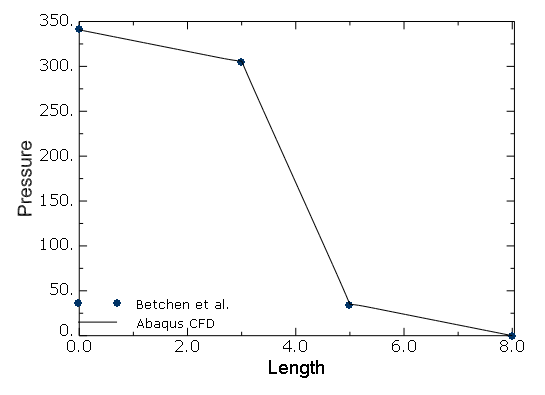
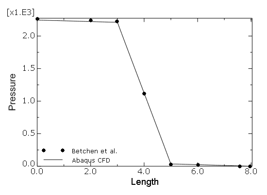
The results of all the cases generated using Abaqus/CFD are compared with the published results of Betchen et al. (2006). For the case of ![]() and
and ![]() , the axial centerline velocity and pressure profiles are shown in Figure 3.3.5–10 and Figure 3.3.5–11 along with the numerical results of Betchen et al. (2006). For
, the axial centerline velocity and pressure profiles are shown in Figure 3.3.5–10 and Figure 3.3.5–11 along with the numerical results of Betchen et al. (2006). For ![]() and
and ![]() , the comparison of the centerline velocity and pressure profiles are shown in Figure 3.3.5–12 and Figure 3.3.5–13. In Figure 3.3.5–14 the centerline velocity profile for the case of
, the comparison of the centerline velocity and pressure profiles are shown in Figure 3.3.5–12 and Figure 3.3.5–13. In Figure 3.3.5–14 the centerline velocity profile for the case of ![]() is compared with that of Betchen et al. (2006).
is compared with that of Betchen et al. (2006).
For all the cases the results compare very well. However, as seen in Figure 3.3.5–14, for the case of ![]() there is a slight deviation between the Abaqus/CFD results and those of Betchen et al. (2006). As noted earlier, in Betchen et al. (2006), a first-order upwind scheme is used for the advection terms, which results in lower accuracy for higher
there is a slight deviation between the Abaqus/CFD results and those of Betchen et al. (2006). As noted earlier, in Betchen et al. (2006), a first-order upwind scheme is used for the advection terms, which results in lower accuracy for higher ![]() ; Abaqus/CFD uses an advection scheme that is spatially second-order accurate for smoothly varying flows.
; Abaqus/CFD uses an advection scheme that is spatially second-order accurate for smoothly varying flows.
Porous plug: ![]() ,
, ![]() with a 100 × 40 mesh (length × height).
with a 100 × 40 mesh (length × height).
Porous plug: ![]() ,
, ![]() with a 200 × 80 mesh (length × height).
with a 200 × 80 mesh (length × height).
Porous plug: ![]() ,
, ![]() with a 100 × 40 mesh (length × height).
with a 100 × 40 mesh (length × height).
Porous plug: ![]() ,
, ![]() with a 200 × 80 mesh (length × height).
with a 200 × 80 mesh (length × height).
Porous plug: ![]() ,
, ![]() with a 200 × 80 mesh (length × height).
with a 200 × 80 mesh (length × height).
Porous plug: ![]() ,
, ![]() with a 400 × 160 mesh (length × height).
with a 400 × 160 mesh (length × height).
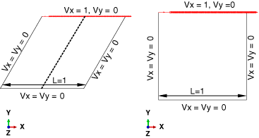
The accuracy of the porous media model is further evaluated using the steady-state flow results for the cases of both orthogonal and skewed fully porous two-dimensional lid-driven cavities at Reynolds numbers of 10 and 1000. The results provided by Krishna et al. (2008), are compared to the Abaqus/CFD results.
The porosity, ![]() , is assumed to be a constant for all the cases; and the aspect ratios for the cavities are set to unity. The Reynolds number, Re, is based on the specified horizontal velocity of the cavity lid,
, is assumed to be a constant for all the cases; and the aspect ratios for the cavities are set to unity. The Reynolds number, Re, is based on the specified horizontal velocity of the cavity lid, ![]() , and the cavity length, L. For
, and the cavity length, L. For ![]() , only orthogonal cavities are considered. Furthermore, Da is set to
, only orthogonal cavities are considered. Furthermore, Da is set to ![]() ,
, ![]() , and
, and ![]() . The porosity
. The porosity ![]() is set to 0.1. For the case of
is set to 0.1. For the case of ![]() , both orthogonal and skewed cavities are considered. The skewed angle is set to 60°. In addition,
, both orthogonal and skewed cavities are considered. The skewed angle is set to 60°. In addition, ![]() and
and ![]() .
.
Model:
The schematics of the skewed and orthogonal two-dimensional cavities used are shown in Figure 3.3.5–15. The two-dimensional problem is solved as an abstraction of the three-dimensional version, and an out-of-plane thickness equal to 0.025 L is specified.
Mesh:
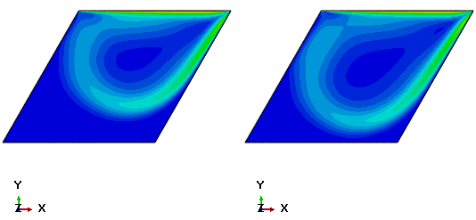
For all the cases a detailed mesh sensitivity analysis is performed by comparing the results of the horizontal and vertical velocity component profiles along the vertical and horizontal geometric centerlines of the cavities, respectively. For Re = 1000, a nonuniform mesh graded near the no-slip/no-penetration boundaries, as shown in Figure 3.3.5–16, was used to resolve the boundary layer and porous media dynamics accurately while reducing the computational time. For the skewed cavity cases the results were particularly sensitive to the boundary layer resolution; a coarser mesh was found to yield incorrect solutions, as shown in Figure 3.3.5–17. Based on these observations, the following conclusions are drawn:
For the cases of Re = 10 and Da = ![]() and
and ![]() , a 64 × 64 uniform mesh was found to be sufficient to obtain mesh independent results.
, a 64 × 64 uniform mesh was found to be sufficient to obtain mesh independent results.
For the case of Re = 10 and Da = ![]() , a 128 × 128 uniform mesh was found to be necessary to obtain mesh independent results.
, a 128 × 128 uniform mesh was found to be necessary to obtain mesh independent results.
For the case of H = 1000 orthogonal cavity, a 64 × 256 nonuniform mesh was necessary to obtain grid independent results.
Similarly, for the case of Re = 1000 and 60° skewed cavity, a 64 × 256 nonuniform mesh was necessary to obtain grid independent results.
Figure 3.3.5–16 Graded mesh used for ![]() orthogonal cavity case. A similar mesh is also used for the 60° skewed cavity case.
orthogonal cavity case. A similar mesh is also used for the 60° skewed cavity case.
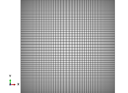
Figure 3.3.5–17 Plot of the steady-state velocity magnitude contours for the case of ![]() ,
, ![]() skewed cavity (60°). Result for a 32 × 128 nonuniform mesh (left) and for a 64 × 256 mesh (right).
skewed cavity (60°). Result for a 32 × 128 nonuniform mesh (left) and for a 64 × 256 mesh (right).
Boundary conditions:
The prescribed boundary conditions are shown in Figure 3.3.5–15. No-slip/no-penetration boundary conditions are applied on the side walls and the base of the cavity by setting the in-plane velocity components ![]() = (0, 0). A constant velocity
= (0, 0). A constant velocity ![]() =
= ![]() = (1, 0) is prescribed at the cavity lid. Furthermore, the two-dimensional nature of the problem is enforced by specifying the out-of-plane z-velocity
= (1, 0) is prescribed at the cavity lid. Furthermore, the two-dimensional nature of the problem is enforced by specifying the out-of-plane z-velocity ![]() on all the boundaries.
on all the boundaries.
If all the flow boundary conditions are prescribed for velocity alone and not for pressure, the solution to the governing equation becomes singular for the pressure unknown. The singularity occurs because any additive constant to pressure would still satisfy both the governing equations (since only the gradient of pressure is involved) and the boundary conditions (since pressure is not involved in their specification). This undetermined additive constant for pressure is the hydrostatic pressure mode and is removed by fixing the value of pressure (either to an arbitrary constant or to a value obtained from experiments) for at least a single point in the domain. In this case p is set to a value of zero at the bottom right corner of the cavity [![]() ].
].
Initial conditions:
At t = 0, the velocity components are set to zero everywhere in the flow domain.
Problem setup:
The following values are used for the flow problem: fluid density ![]() = 1 kg/m3, cavity edge length L = 1 m, and lid velocity
= 1 kg/m3, cavity edge length L = 1 m, and lid velocity ![]() = 1 m/s. To vary the Reynolds number, the dynamic viscosity
= 1 m/s. To vary the Reynolds number, the dynamic viscosity ![]() is changed, as given in Table 3.3.5–4. Since the length scale
is changed, as given in Table 3.3.5–4. Since the length scale ![]() , the permeability
, the permeability ![]() . Thus, for the case of
. Thus, for the case of ![]() ,
, ![]() ,
, ![]() , and
, and ![]() . For the case of
. For the case of ![]() ,
, ![]() .
.
To achieve a steady state, a backward Euler time integration scheme (the time weights ![]() for all the discretized terms) is used with the implicit advection scheme and the CFL number set to 40. It is observed that for such high CFL numbers, the default momentum solver—the Diagonally Scaled Flexible Generalized Minimum Residual linear solver (DSFGMRES)—results either in poor convergence or in some cases nonconvergence. Hence, the momentum solver type is set to the Incomplete LU factorization preconditioned Flexible Generalized Minimum Residual linear solver (ILUFGMRES), which results in good convergence for all cases. All other solver options are set to the default values. Various smaller CFL numbers down to 0.45 are also tested with both the backward Euler and the Crank-Nicolson time integration schemes and with an explicit advection scheme. The steady-state solutions are found to be invariant with respect to these settings.
for all the discretized terms) is used with the implicit advection scheme and the CFL number set to 40. It is observed that for such high CFL numbers, the default momentum solver—the Diagonally Scaled Flexible Generalized Minimum Residual linear solver (DSFGMRES)—results either in poor convergence or in some cases nonconvergence. Hence, the momentum solver type is set to the Incomplete LU factorization preconditioned Flexible Generalized Minimum Residual linear solver (ILUFGMRES), which results in good convergence for all cases. All other solver options are set to the default values. Various smaller CFL numbers down to 0.45 are also tested with both the backward Euler and the Crank-Nicolson time integration schemes and with an explicit advection scheme. The steady-state solutions are found to be invariant with respect to these settings.
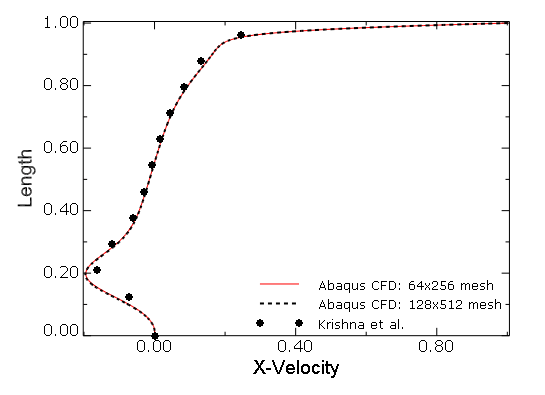
The results of Abaqus/CFD are compared with the published results of Krishna et al. (2008). In Figure 3.3.5–18 and Figure 3.3.5–19 the comparison results of the horizontal and vertical velocity component profiles along the vertical and horizontal geometric centerlines of the cavities for the cases of ![]() and
and ![]() and
and ![]() are shown. The results are in excellent agreement with the published results. These results are also in very good agreement with the Lattice-Boltzmann simulation results of Guo and Zhao (2002) (results not shown). The comparison results of the horizontal component of the velocity profile along the vertical centerline for the case of the
are shown. The results are in excellent agreement with the published results. These results are also in very good agreement with the Lattice-Boltzmann simulation results of Guo and Zhao (2002) (results not shown). The comparison results of the horizontal component of the velocity profile along the vertical centerline for the case of the ![]() orthogonal cavity and
orthogonal cavity and ![]() are shown in Figure 3.3.5–20, along with the results obtained using different meshes. For the 60° skewed cavity and
are shown in Figure 3.3.5–20, along with the results obtained using different meshes. For the 60° skewed cavity and ![]() , the results for the horizontal component of the velocity profile along the geometric centerline (see Figure 3.3.5–15) are shown in Figure 3.3.5–21, along with the results obtained using different meshes. The results for
, the results for the horizontal component of the velocity profile along the geometric centerline (see Figure 3.3.5–15) are shown in Figure 3.3.5–21, along with the results obtained using different meshes. The results for ![]() are seen to deviate slightly from those of Krishna et al. (2008), near the bottom of the cavity, although the grid independence study in Krishna et al. (2008), considers the maximum streamline value, which occurs near the top of the cavity, as the convergence metric. Based on such a metric, a uniform 120 × 120 mesh was used in their simulations. A better metric would have been to use the minimum horizontal component of the velocity along the geometric centerline since it was noted from Abaqus/CFD simulations that this quantity is slower to converge than the maximum streamline values that converge even on coarser meshes.
are seen to deviate slightly from those of Krishna et al. (2008), near the bottom of the cavity, although the grid independence study in Krishna et al. (2008), considers the maximum streamline value, which occurs near the top of the cavity, as the convergence metric. Based on such a metric, a uniform 120 × 120 mesh was used in their simulations. A better metric would have been to use the minimum horizontal component of the velocity along the geometric centerline since it was noted from Abaqus/CFD simulations that this quantity is slower to converge than the maximum streamline values that converge even on coarser meshes.
Figure 3.3.5–18 Comparison of profiles for the horizontal component of velocity along the vertical centerline of the orthogonal cavity (![]() and
and ![]() and
and ![]() ).
).
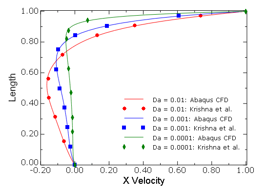
Figure 3.3.5–19 Comparison of profiles for the vertical component of velocity along the horizontal centerline of the orthogonal cavity (![]() and
and ![]() and
and ![]() ).
).
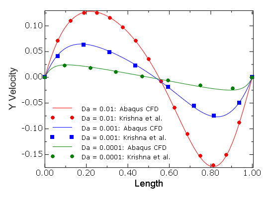
Figure 3.3.5–20 Comparison of profiles for the horizontal component of velocity along the vertical centerline (![]() and
and ![]() ; orthogonal cavity).
; orthogonal cavity).
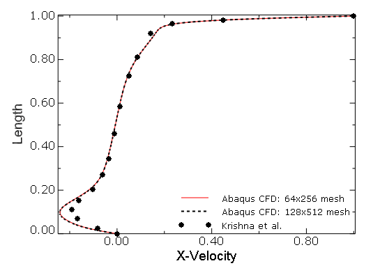
Figure 3.3.5–21 Comparison of profiles for the horizontal component of velocity along the geometric centerline (![]() and
and ![]()
![]() ; skewed cavity)—see Figure 3.3.5–15.
; skewed cavity)—see Figure 3.3.5–15.
Fully porous orthogonal lid-driven cavity: ![]() ,
, ![]() with a 64 × 64 uniform mesh.
with a 64 × 64 uniform mesh.
Fully porous orthogonal lid-driven cavity: ![]() ,
, ![]() with a 64 × 64 uniform mesh.
with a 64 × 64 uniform mesh.
Fully porous orthogonal lid-driven cavity: ![]() ,
, ![]() with a 64 × 64 uniform mesh.
with a 64 × 64 uniform mesh.
Fully porous orthogonal lid-driven cavity: ![]() ,
, ![]() with a 128 × 128 uniform mesh.
with a 128 × 128 uniform mesh.
Fully porous orthogonal lid-driven cavity: ![]() ,
, ![]() with 3481 elements nonuniform mesh.
with 3481 elements nonuniform mesh.
Fully porous orthogonal lid-driven cavity: ![]() ,
, ![]() with 13924 elements nonuniform mesh.
with 13924 elements nonuniform mesh.
Fully porous orthogonal lid-driven cavity: ![]() ,
, ![]() with 56169 elements nonuniform mesh.
with 56169 elements nonuniform mesh.
Fully porous 60° skewed lid-driven cavity: ![]() ,
, ![]() with 3481 elements nonuniform mesh.
with 3481 elements nonuniform mesh.
Fully porous 60° skewed lid-driven cavity: ![]() ,
, ![]() with 13924 elements nonuniform mesh.
with 13924 elements nonuniform mesh.
Fully porous 60° skewed lid-driven cavity: ![]() ,
, ![]() with 56169 elements nonuniform mesh.
with 56169 elements nonuniform mesh.
Guo, Z., and T. S. Zhao, “Lattice Boltzmann Model for Incompressible Flows through Porous Media,” Physical Review E, vol. 66, pp. 036304 (1–9), 2002.
Krishna, J. D., T. Basak, and S. K. Das, “Numerical Study of Lid-Driven Flow in Orthogonal and Skewed Porous Cavity,” Communication in Numerical Methods in Engineering, vol. 24, pp. 815–831, 2008.
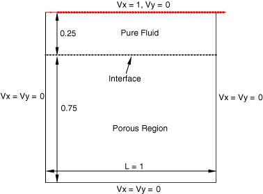
The accuracy of the porous media model is further evaluated using the steady-state flow results for the cases of an orthogonal partially porous two-dimensional lid-driven cavity at ![]() and
and ![]() ,
, ![]() , and
, and ![]() . The results provided by Bai et al. (2009), are compared to the Abaqus/CFD results.
. The results provided by Bai et al. (2009), are compared to the Abaqus/CFD results.
The porosity ![]() for all the cases considered, and the aspect ratio of the orthogonal cavity is set to unity. The Reynolds number, Re, is based on the specified horizontal velocity of the cavity lid,
for all the cases considered, and the aspect ratio of the orthogonal cavity is set to unity. The Reynolds number, Re, is based on the specified horizontal velocity of the cavity lid, ![]() , and the cavity length, L.
, and the cavity length, L.
Model:
The geometry of the two-dimensional partially porous orthogonal cavity used is shown in Figure 3.3.5–22. The length of the domain, L, is set equal to 1. The pure fluid region occupies the top quarter of the domain, while the remaining volume is occupied by the porous medium. The two-dimensional problem is solved as an abstraction of the three-dimensional version, and an out-of-plane thickness equal to 0.01L is specified.
Mesh:
For all the cases considered, a detailed mesh sensitivity analysis is performed by comparing the horizontal and vertical velocity component profiles along the vertical and horizontal geometric centerlines of the cavities. For all the cases a 64 × 64 uniform mesh was found sufficient to produce mesh independent results. The out-of-plane dimension (z-axis) is meshed with only one element to enforce the two-dimensional nature of the problem.
Boundary conditions:
The prescribed boundary conditions are shown in Figure 3.3.5–22. No-slip/no-penetration boundary conditions are applied on the side walls and the base of the cavity by setting the in-plane velocity components ![]() = (0, 0). A constant velocity
= (0, 0). A constant velocity ![]() =
= ![]() = (1, 0) is prescribed at the cavity lid. Furthermore, the two-dimensional nature of the problem is enforced by specifying the out-of-plane z-velocity
= (1, 0) is prescribed at the cavity lid. Furthermore, the two-dimensional nature of the problem is enforced by specifying the out-of-plane z-velocity ![]() everywhere in the domain.
everywhere in the domain.
If all the flow boundary conditions are prescribed for velocity alone and not for pressure, the solution to the governing equation becomes singular for the pressure unknown because any additive constant to pressure would still satisfy both the governing equations (since only the gradient of pressure is involved) and the boundary conditions (since pressure is not involved in their specification). This undetermined additive constant for pressure is the hydrostatic pressure mode and is removed by fixing the value of pressure (either to an arbitrary constant or to a value obtained from experiments) for at least a single point in the domain. In this case p is set to a value of zero at the bottom right corner of the cavity [![]() ].
].
Initial conditions:
At t = 0, the velocity components are set to zero everywhere in the flow domain.
Problem setup:
The following values are used for the flow problem: fluid density ![]() 1 kg/m3, dynamic viscosity,
1 kg/m3, dynamic viscosity, ![]() kg/m/s, cavity edge length L = 1 m, and lid velocity
kg/m/s, cavity edge length L = 1 m, and lid velocity ![]() =1 m/s. Since the length scale
=1 m/s. Since the length scale ![]() , the permeability
, the permeability ![]() and, hence,
and, hence, ![]() ,
, ![]() , and
, and ![]() .
.
To achieve a steady state, a backward Euler time integration scheme (the time weights ![]() for all the discretized terms) is used with the implicit advection scheme and the CFL number set to 40. It was observed that for such high CFL numbers, the default momentum solver (DSFGMRES) resulted either in poor convergence or in some cases nonconvergence. Hence, the momentum solver type was set to ILUFGMRES, which resulted in good convergence for all cases. All other solver options are set to the default values. Various smaller CFL numbers down to 0.45 were also tested with both the backward Euler and the Crank-Nicolson time integration schemes and with an explicit advection scheme. The steady-state solutions were found to be invariant with respect to these settings.
for all the discretized terms) is used with the implicit advection scheme and the CFL number set to 40. It was observed that for such high CFL numbers, the default momentum solver (DSFGMRES) resulted either in poor convergence or in some cases nonconvergence. Hence, the momentum solver type was set to ILUFGMRES, which resulted in good convergence for all cases. All other solver options are set to the default values. Various smaller CFL numbers down to 0.45 were also tested with both the backward Euler and the Crank-Nicolson time integration schemes and with an explicit advection scheme. The steady-state solutions were found to be invariant with respect to these settings.
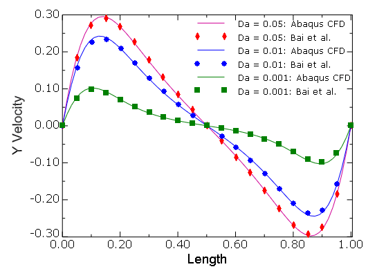
The results of Abaqus/CFD are compared with the published results of Bai et al. (2009). In Figure 3.3.5–23 and Figure 3.3.5–24 the comparison results of the horizontal and vertical velocity component profiles along the vertical and horizontal geometric centerlines of the cavities for the cases of ![]() and
and ![]() and
and ![]() are shown. The results are in excellent agreement with the published results.
are shown. The results are in excellent agreement with the published results.
Figure 3.3.5–23 Comparison of profiles for the horizontal component of velocity along the vertical centerline of the orthogonal cavity (![]() and
and ![]() and
and ![]() ).
).
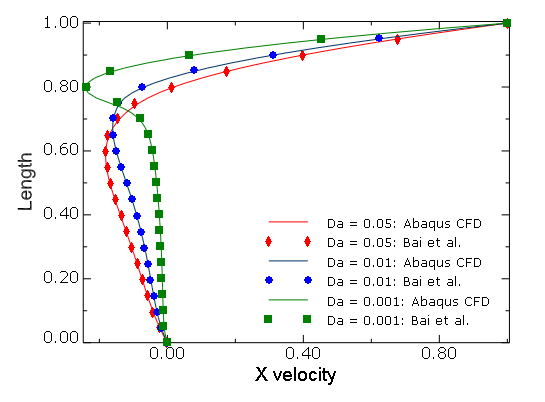
Figure 3.3.5–24 Comparison of profiles for the vertical component of velocity along the horizontal interface between the porous and pure fluid region (![]() and
and ![]() and
and ![]() )—see Figure 3.3.5–22.
)—see Figure 3.3.5–22.
Partially porous orthogonal lid-driven cavity: ![]() ,
, ![]() with a 64 × 64 uniform mesh.
with a 64 × 64 uniform mesh.
Partially porous orthogonal lid-driven cavity: ![]() ,
, ![]() with a 64 × 64 uniform mesh.
with a 64 × 64 uniform mesh.
Partially porous orthogonal lid -driven cavity: ![]() ,
, ![]() with a 64 × 64 uniform mesh.
with a 64 × 64 uniform mesh.